Inotersen (Yu 2020) • nlmixr2lib

library(nlmixr2lib)
library(rxode2)
#> rxode2 5.1.8 using 2 threads (see ?getRxThreads)
#>   no cache: create with `rxCreateCache()`
library(dplyr)
#> 
#> Attaching package: 'dplyr'
#> The following objects are masked from 'package:stats':
#> 
#>     filter, lag
#> The following objects are masked from 'package:base':
#> 
#>     intersect, setdiff, setequal, union
library(tidyr)
library(ggplot2)
library(PKNCA)
#> 
#> Attaching package: 'PKNCA'
#> The following object is masked from 'package:stats':
#> 
#>     filter

Inotersen population PK/PD in hATTR polyneuropathy (Yu 2020)

Yu et al. (2020) developed the first population PK/PD model for an antisense oligonucleotide therapeutic: inotersen, a 20-mer 2’-O-methoxyethyl gapmer that reduces hepatic production of transthyretin (TTR). Plasma inotersen follows a two-compartment model with first-order SC absorption and linear elimination from the central compartment. Serum TTR follows an indirect-response model in which inotersen inhibits the zero-order production of TTR:

$\frac{dTTR}{dt} = k_{in}\left(1 - \frac{I_{max} C_p}{IC_{50} + C_p}\right) - k_{out}\,TTR$

with $k_{in} = BL \cdot k_{out}$ so that TTR starts at its baseline. The PK model was fit first and the individual (post hoc) PK parameters then drove the PD fit; the packaged model carries both layers in one file.

Citation: Yu RZ, Collins JW, Hall S, Ackermann EJ, Geary RS, Monia BP, Henry SP, Wang Y. Population Pharmacokinetic-Pharmacodynamic Modeling of Inotersen, an Antisense Oligonucleotide for Treatment of Patients with Hereditary Transthyretin Amyloidosis. Nucleic Acid Ther. 2020;30(3):153-163. doi:10.1089/nat.2019.0822
Article: https://doi.org/10.1089/nat.2019.0822

Population

The analysis pooled three Ionis studies (Yu 2020 Clinical studies section and Table 1): a phase 1 single- and multiple-ascending-dose study in 51 inotersen-treated healthy volunteers (50-400 mg SC), the pivotal phase 2/3 NEURO-TTR study (300 mg SC on days 1, 3 and 5 then once weekly for 65 weeks) and its open-label extension (300 mg SC weekly for up to 5 years). Of 202 subjects, 151 were patients with hereditary transthyretin amyloidosis with polyneuropathy (hATTR-PN); 197 contributed 3,602 PK observations. Median age was 57 years (range 25-81), median body weight 71.8 kg (37.0-140), median lean body mass 51.6 kg (31.3-80.3), 69.8% were male, and 87.6% were Caucasian, 7.43% African American and 3.47% Asian. Median baseline TTR was 22.1 mg/dL. PK samples collected after the onset of antidrug antibodies were excluded.

The same information is available programmatically via readModelDb("Yu_2020_inotersen")()$population.

Source trace

Every ini() value carries an in-file comment naming its source row. They are collected here for review.

Parameter / equation	Value	Source
`ka`	0.261 1/h	Table 2 ‘Absorption rate constant, Ka’
`CL/F` (hATTR, LBM 51.6 kg)	3.4 L/h	Table 2 ‘Clearance, CL’
`Vc/F` (hATTR, LBM 51.6 kg)	20.7 L	Table 2 ‘Central volume, Vc’
`Q/F`	0.266 L/h	Table 2 ‘Intercompartmental clearance, Q’
`Vp/F`	230 L	Table 2 ‘Peripheral volume, Vp’
LBM exponent on CL/F and Q/F	1 (fixed)	Table 2 ‘Lean body mass * CL/Q’, power centred on median
LBM exponent on Vc/F and Vp/F	1 (fixed)	Table 2 ‘Lean body mass * Vc/Vp’, power centred on median
LBM reference	51.6 kg	Table 1 lean body mass median
Healthy effect on CL/F	+0.111, `(1 + 0.111 * DIS_HEALTHY)`	Table 2 ‘Disease * CL’, proportional
Healthy effect on Vc/F	-0.284, `(1 - 0.284 * DIS_HEALTHY)`	Table 2 ‘Disease * Vc’, proportional
omega^2 CL, Vc, Vp	0.071, 0.335, 0.677	Table 2
cov(Vc, CL), cov(CL, Vp)	0.049, -0.145	Table 2 (cov(Vc, Vp) not reported; set to 0)
PK residual	sigma^2 = 0.168 log-additive; `expSd = sqrt(0.168) = 0.4099`	Table 2
`Imax`	0.913	Table 3
`IC50`	9.07 ng/mL	Table 3
Baseline TTR (hATTR)	20.4 mg/dL	Table 3 ‘Estimated baseline’
Healthy effect on baseline	+0.269, `(1 + 0.269 * DIS_HEALTHY)`	Table 3 and its footnote
`kout`	0.00308 1/h	Table 3
omega^2 IC50, kout; cov	0.953, 0.288; -0.182	Table 3
omega^2 baseline	0.0537	Table 3
PD residual	proportional 0.13, additive 1.35 mg/dL	Table 3 ‘Residual variability (log space), (SD)’
Indirect-response equation	see above	Population PD modeling section

Covariates

Source	Canonical column	Notes
Lean body mass (kg)	`LBM`	Reference 51.6 kg. The paper does not state which LBM formula it used.
Disease status	`DIS_HEALTHY`	1 = healthy volunteer, 0 = hATTR-PN patient (reference).

Closed-form checks on the typical PK

The paper derives four numbers from its typical PK estimates: alpha and beta half-lives of 3.91 h and 26.9 days, a steady-state volume of 250.7 L, and a trough accumulation ratio of 6.07 for weekly dosing. These use the same parameters on both sides, so they are checked tightly.

ini_df <- rxode2::rxode2(readModelDb("Yu_2020_inotersen"))$iniDf
#> ℹ parameter labels from comments will be replaced by 'label()'
th <- setNames(ini_df$est, ini_df$name)
cl <- exp(th[["lcl"]])
vc <- exp(th[["lvc"]])
q <- exp(th[["lq"]])
vp <- exp(th[["lvp"]])
kel <- cl / vc
k12 <- q / vc
k21 <- q / vp
s <- kel + k12 + k21
alpha <- (s + sqrt(s^2 - 4 * kel * k21)) / 2
beta <- (s - sqrt(s^2 - 4 * kel * k21)) / 2
checks <- data.frame(
  Quantity = c(
    "Alpha half-life (h)",
    "Beta half-life (days)",
    "Vss (L)",
    "Trough accumulation ratio, QW"
  ),
  Paper = c(3.91, 26.9, 250.7, 6.07),
  Model = c(
    log(2) / alpha,
    log(2) / beta / 24,
    vc + vp,
    1 / (1 - exp(-beta * 168))
  )
)
knitr::kable(checks, digits = 3)

Quantity	Paper	Model
Alpha half-life (h)	3.91	3.912
Beta half-life (days)	26.90	26.939
Vss (L)	250.70	250.700
Trough accumulation ratio, QW	6.07	6.067

stopifnot(all(abs(checks$Model / checks$Paper - 1) < 0.01))

Virtual cohort and dosing regimens

Yu 2020 simulated the 151 hATTR-PN patients of the analysis dataset under four regimens for 65 weeks (Simulations section). Subject-level covariates are not published, so the virtual cohort below draws lean body mass from a truncated log-normal around the pooled-cohort median and range (Table 1); all subjects are patients (DIS_HEALTHY = 0). Each regimen uses the same 150 virtual patients so that differences between arms come from the dosing alone.

Day 1 of the paper is time 0, so day d is (d - 1) * 24 h; the last dose of each regimen falls on day 449 (t = 10752 h), which is where Table 4 reports the steady-state interval.

set.seed(20200301)
rxode2::rxSetSeed(20200301)
n_per_arm <- 150L

cohort <- tibble(
  subj = seq_len(n_per_arm),
  LBM = pmin(pmax(rlnorm(n_per_arm, log(51.6), 0.16), 31.3), 80.3),
  DIS_HEALTHY = 0L
)

t_last <- 448 * 24
regimens <- list(
  "300 mg QW" = list(amt = 300, times = seq(0, t_last, by = 168), tau = 168),
  "300 mg QOW" = list(amt = 300, times = seq(0, t_last, by = 336), tau = 336),
  "Loading + 300 mg QW" = list(
    amt = 300,
    times = c(0, 48, 96, seq(168, t_last, by = 168)),
    tau = 168
  ),
  "150 mg QW" = list(amt = 150, times = seq(0, t_last, by = 168), tau = 168)
)

make_arm <- function(arm_index, cohort, regimens) {
  reg <- regimens[[arm_index]]
  ids <- cohort |> mutate(id = subj + (arm_index - 1L) * nrow(cohort))
  dense <- c(seq(0, 12, by = 0.5), seq(14, reg$tau, by = 2))
  obs_t <- sort(unique(c(
    dense,
    seq(0, t_last + reg$tau, by = 24),
    t_last + dense
  )))
  doses <- ids |>
    crossing(time = reg$times) |>
    mutate(amt = reg$amt, evid = 1L, cmt = "depot", dvid = NA_integer_)
  obs <- ids |>
    crossing(time = obs_t) |>
    mutate(amt = 0, evid = 0L, cmt = NA_character_, dvid = 1L)
  bind_rows(doses, obs) |>
    mutate(regimen = names(regimens)[arm_index], tau = reg$tau) |>
    arrange(id, time, desc(evid))
}

events <- bind_rows(lapply(
  seq_along(regimens),
  make_arm,
  cohort = cohort,
  regimens = regimens
))
stopifnot(!anyDuplicated(events[, c("id", "time", "evid")]))

Simulation

The model has two endpoints (Cc and ttr), so observation rows carry dvid = 1 with no compartment; rxode2 returns both outputs at every observation time. Residual error is not added (sigma = NA); between-subject variability is simulated.

mod <- readModelDb("Yu_2020_inotersen")
sim <- rxode2::rxSolve(
  mod,
  events = events,
  sigma = NA,
  useLinCmt = FALSE,
  keep = c("regimen", "tau"),
  returnType = "data.frame"
)
#> ℹ parameter labels from comments will be replaced by 'label()'
sim <- sim |> mutate(regimen = factor(regimen, levels = names(regimens)))

Replicate published figures

Figure 4: plasma trough concentrations

trough <- sim |>
  filter(time %in% seq(168, t_last + 336, by = 168)) |>
  group_by(regimen, time) |>
  summarise(
    Q05 = quantile(Cc, 0.05),
    Q50 = median(Cc),
    Q95 = quantile(Cc, 0.95),
    .groups = "drop"
  )

ggplot(trough, aes(time / 24 / 7, Q50, colour = regimen, fill = regimen)) +
  geom_ribbon(aes(ymin = Q05, ymax = Q95), alpha = 0.15, colour = NA) +
  geom_line(linewidth = 0.8) +
  labs(
    x = "Time (weeks)",
    y = "Inotersen plasma trough (ng/mL)",
    colour = NULL,
    fill = NULL,
    caption = "Replicates Figure 4 of Yu 2020 (median and 90% prediction interval)."
  ) +
  theme_bw()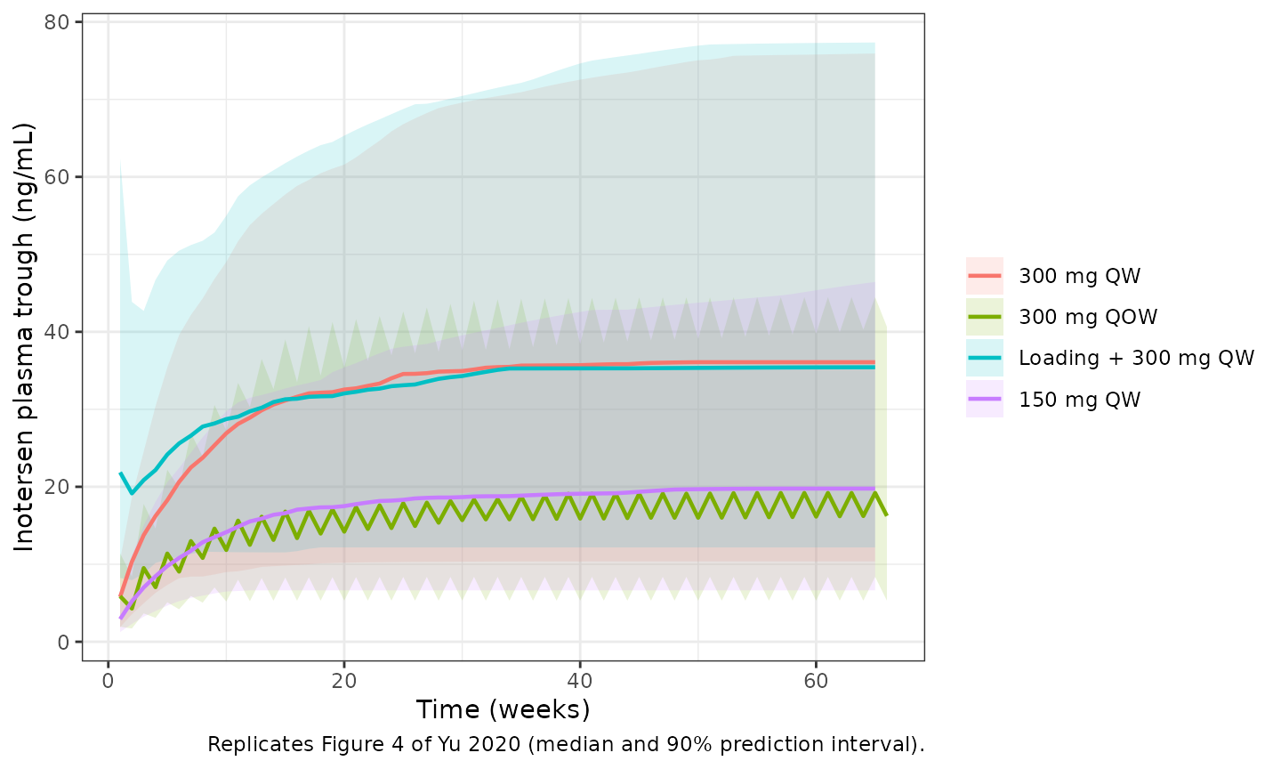

Figure 5: serum TTR

ttr_prof <- sim |>
  filter(time %% 24 == 0) |>
  group_by(regimen, time) |>
  summarise(
    Q05 = quantile(ttr, 0.05),
    Q50 = median(ttr),
    Q95 = quantile(ttr, 0.95),
    .groups = "drop"
  )

ggplot(ttr_prof, aes(time / 24 / 7, Q50, colour = regimen, fill = regimen)) +
  geom_ribbon(aes(ymin = Q05, ymax = Q95), alpha = 0.12, colour = NA) +
  geom_line(linewidth = 0.8) +
  labs(
    x = "Time (weeks)",
    y = "Serum TTR (mg/dL)",
    colour = NULL,
    fill = NULL,
    caption = "Replicates Figure 5 of Yu 2020 (median and 90% prediction interval)."
  ) +
  theme_bw()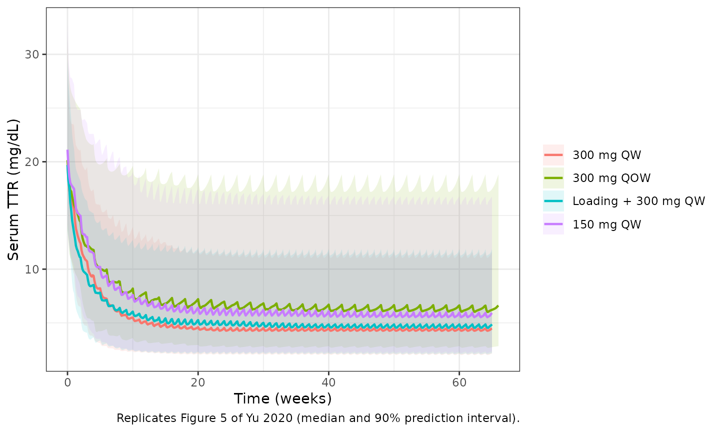

PKNCA validation against Table 4

Table 4 reports geometric means of AUC over the dosing interval, Cmax and Ctrough after the first dose (day 1) and after the last dose (day 449). NCA is run on both intervals for each regimen, with Ctrough taken as the concentration at the end of the interval (PKNCA ctrough), i.e. just before the next dose. For the loading regimen the day-1 interval is not compared, because the paper’s day-1 values for that arm mix a 48-hour trough with an AUC equal to the weekly arms’ and the interval it used is not stated.

# Each interval is re-anchored to its own dose so that it starts at time 0:
# PKNCA evaluates ctrough on time after dose, and the two periods are then
# separate PKNCA groups.
tau_by_reg <- vapply(regimens, `[[`, numeric(1), "tau")
periods <- c("Day 1" = 0, "Day 449" = t_last)

conc <- bind_rows(lapply(names(periods), function(p) {
  sim |>
    filter(!is.na(Cc)) |>
    mutate(time = time - periods[[p]], period = p) |>
    filter(time >= 0, time <= tau_by_reg[as.character(regimen)])
})) |>
  mutate(regimen = as.character(regimen)) |>
  select(id, time, Cc, regimen, period)

doses <- bind_rows(lapply(names(periods), function(p) {
  events |>
    filter(evid == 1L) |>
    mutate(time = time - periods[[p]], period = p) |>
    filter(time >= 0, time < tau)
})) |>
  select(id, time, amt, regimen, period)

intervals <- expand.grid(
  regimen = names(regimens),
  period = names(periods),
  stringsAsFactors = FALSE
) |>
  mutate(start = 0, end = unname(tau_by_reg[regimen])) |>
  filter(!(regimen == "Loading + 300 mg QW" & period == "Day 1")) |>
  mutate(auclast = TRUE, cmax = TRUE, ctrough = TRUE)

nca <- PKNCA::pk.nca(PKNCA::PKNCAdata(
  PKNCA::PKNCAconc(conc, Cc ~ time | regimen + period + id),
  PKNCA::PKNCAdose(doses, amt ~ time | regimen + period + id),
  intervals = intervals
))
#> Warning: regimen=Loading + 300 mg QW; period=Day 1; id=301: No intervals for
#> data
#> Warning: regimen=Loading + 300 mg QW; period=Day 1; id=302: No intervals for
#> data
#> Warning: regimen=Loading + 300 mg QW; period=Day 1; id=303: No intervals for
#> data
#> Warning: regimen=Loading + 300 mg QW; period=Day 1; id=304: No intervals for
#> data
#> Warning: regimen=Loading + 300 mg QW; period=Day 1; id=305: No intervals for
#> data
#> Warning: regimen=Loading + 300 mg QW; period=Day 1; id=306: No intervals for
#> data
#> Warning: regimen=Loading + 300 mg QW; period=Day 1; id=307: No intervals for
#> data
#> Warning: regimen=Loading + 300 mg QW; period=Day 1; id=308: No intervals for
#> data
#> Warning: regimen=Loading + 300 mg QW; period=Day 1; id=309: No intervals for
#> data
#> Warning: regimen=Loading + 300 mg QW; period=Day 1; id=310: No intervals for
#> data
#> Warning: regimen=Loading + 300 mg QW; period=Day 1; id=311: No intervals for
#> data
#> Warning: regimen=Loading + 300 mg QW; period=Day 1; id=312: No intervals for
#> data
#> Warning: regimen=Loading + 300 mg QW; period=Day 1; id=313: No intervals for
#> data
#> Warning: regimen=Loading + 300 mg QW; period=Day 1; id=314: No intervals for
#> data
#> Warning: regimen=Loading + 300 mg QW; period=Day 1; id=315: No intervals for
#> data
#> Warning: regimen=Loading + 300 mg QW; period=Day 1; id=316: No intervals for
#> data
#> Warning: regimen=Loading + 300 mg QW; period=Day 1; id=317: No intervals for
#> data
#> Warning: regimen=Loading + 300 mg QW; period=Day 1; id=318: No intervals for
#> data
#> Warning: regimen=Loading + 300 mg QW; period=Day 1; id=319: No intervals for
#> data
#> Warning: regimen=Loading + 300 mg QW; period=Day 1; id=320: No intervals for
#> data
#> Warning: regimen=Loading + 300 mg QW; period=Day 1; id=321: No intervals for
#> data
#> Warning: regimen=Loading + 300 mg QW; period=Day 1; id=322: No intervals for
#> data
#> Warning: regimen=Loading + 300 mg QW; period=Day 1; id=323: No intervals for
#> data
#> Warning: regimen=Loading + 300 mg QW; period=Day 1; id=324: No intervals for
#> data
#> Warning: regimen=Loading + 300 mg QW; period=Day 1; id=325: No intervals for
#> data
#> Warning: regimen=Loading + 300 mg QW; period=Day 1; id=326: No intervals for
#> data
#> Warning: regimen=Loading + 300 mg QW; period=Day 1; id=327: No intervals for
#> data
#> Warning: regimen=Loading + 300 mg QW; period=Day 1; id=328: No intervals for
#> data
#> Warning: regimen=Loading + 300 mg QW; period=Day 1; id=329: No intervals for
#> data
#> Warning: regimen=Loading + 300 mg QW; period=Day 1; id=330: No intervals for
#> data
#> Warning: regimen=Loading + 300 mg QW; period=Day 1; id=331: No intervals for
#> data
#> Warning: regimen=Loading + 300 mg QW; period=Day 1; id=332: No intervals for
#> data
#> Warning: regimen=Loading + 300 mg QW; period=Day 1; id=333: No intervals for
#> data
#> Warning: regimen=Loading + 300 mg QW; period=Day 1; id=334: No intervals for
#> data
#> Warning: regimen=Loading + 300 mg QW; period=Day 1; id=335: No intervals for
#> data
#> Warning: regimen=Loading + 300 mg QW; period=Day 1; id=336: No intervals for
#> data
#> Warning: regimen=Loading + 300 mg QW; period=Day 1; id=337: No intervals for
#> data
#> Warning: regimen=Loading + 300 mg QW; period=Day 1; id=338: No intervals for
#> data
#> Warning: regimen=Loading + 300 mg QW; period=Day 1; id=339: No intervals for
#> data
#> Warning: regimen=Loading + 300 mg QW; period=Day 1; id=340: No intervals for
#> data
#> Warning: regimen=Loading + 300 mg QW; period=Day 1; id=341: No intervals for
#> data
#> Warning: regimen=Loading + 300 mg QW; period=Day 1; id=342: No intervals for
#> data
#> Warning: regimen=Loading + 300 mg QW; period=Day 1; id=343: No intervals for
#> data
#> Warning: regimen=Loading + 300 mg QW; period=Day 1; id=344: No intervals for
#> data
#> Warning: regimen=Loading + 300 mg QW; period=Day 1; id=345: No intervals for
#> data
#> Warning: regimen=Loading + 300 mg QW; period=Day 1; id=346: No intervals for
#> data
#> Warning: regimen=Loading + 300 mg QW; period=Day 1; id=347: No intervals for
#> data
#> Warning: regimen=Loading + 300 mg QW; period=Day 1; id=348: No intervals for
#> data
#> Warning: regimen=Loading + 300 mg QW; period=Day 1; id=349: No intervals for
#> data
#> Warning: regimen=Loading + 300 mg QW; period=Day 1; id=350: No intervals for
#> data
#> Warning: regimen=Loading + 300 mg QW; period=Day 1; id=351: No intervals for
#> data
#> Warning: regimen=Loading + 300 mg QW; period=Day 1; id=352: No intervals for
#> data
#> Warning: regimen=Loading + 300 mg QW; period=Day 1; id=353: No intervals for
#> data
#> Warning: regimen=Loading + 300 mg QW; period=Day 1; id=354: No intervals for
#> data
#> Warning: regimen=Loading + 300 mg QW; period=Day 1; id=355: No intervals for
#> data
#> Warning: regimen=Loading + 300 mg QW; period=Day 1; id=356: No intervals for
#> data
#> Warning: regimen=Loading + 300 mg QW; period=Day 1; id=357: No intervals for
#> data
#> Warning: regimen=Loading + 300 mg QW; period=Day 1; id=358: No intervals for
#> data
#> Warning: regimen=Loading + 300 mg QW; period=Day 1; id=359: No intervals for
#> data
#> Warning: regimen=Loading + 300 mg QW; period=Day 1; id=360: No intervals for
#> data
#> Warning: regimen=Loading + 300 mg QW; period=Day 1; id=361: No intervals for
#> data
#> Warning: regimen=Loading + 300 mg QW; period=Day 1; id=362: No intervals for
#> data
#> Warning: regimen=Loading + 300 mg QW; period=Day 1; id=363: No intervals for
#> data
#> Warning: regimen=Loading + 300 mg QW; period=Day 1; id=364: No intervals for
#> data
#> Warning: regimen=Loading + 300 mg QW; period=Day 1; id=365: No intervals for
#> data
#> Warning: regimen=Loading + 300 mg QW; period=Day 1; id=366: No intervals for
#> data
#> Warning: regimen=Loading + 300 mg QW; period=Day 1; id=367: No intervals for
#> data
#> Warning: regimen=Loading + 300 mg QW; period=Day 1; id=368: No intervals for
#> data
#> Warning: regimen=Loading + 300 mg QW; period=Day 1; id=369: No intervals for
#> data
#> Warning: regimen=Loading + 300 mg QW; period=Day 1; id=370: No intervals for
#> data
#> Warning: regimen=Loading + 300 mg QW; period=Day 1; id=371: No intervals for
#> data
#> Warning: regimen=Loading + 300 mg QW; period=Day 1; id=372: No intervals for
#> data
#> Warning: regimen=Loading + 300 mg QW; period=Day 1; id=373: No intervals for
#> data
#> Warning: regimen=Loading + 300 mg QW; period=Day 1; id=374: No intervals for
#> data
#> Warning: regimen=Loading + 300 mg QW; period=Day 1; id=375: No intervals for
#> data
#> Warning: regimen=Loading + 300 mg QW; period=Day 1; id=376: No intervals for
#> data
#> Warning: regimen=Loading + 300 mg QW; period=Day 1; id=377: No intervals for
#> data
#> Warning: regimen=Loading + 300 mg QW; period=Day 1; id=378: No intervals for
#> data
#> Warning: regimen=Loading + 300 mg QW; period=Day 1; id=379: No intervals for
#> data
#> Warning: regimen=Loading + 300 mg QW; period=Day 1; id=380: No intervals for
#> data
#> Warning: regimen=Loading + 300 mg QW; period=Day 1; id=381: No intervals for
#> data
#> Warning: regimen=Loading + 300 mg QW; period=Day 1; id=382: No intervals for
#> data
#> Warning: regimen=Loading + 300 mg QW; period=Day 1; id=383: No intervals for
#> data
#> Warning: regimen=Loading + 300 mg QW; period=Day 1; id=384: No intervals for
#> data
#> Warning: regimen=Loading + 300 mg QW; period=Day 1; id=385: No intervals for
#> data
#> Warning: regimen=Loading + 300 mg QW; period=Day 1; id=386: No intervals for
#> data
#> Warning: regimen=Loading + 300 mg QW; period=Day 1; id=387: No intervals for
#> data
#> Warning: regimen=Loading + 300 mg QW; period=Day 1; id=388: No intervals for
#> data
#> Warning: regimen=Loading + 300 mg QW; period=Day 1; id=389: No intervals for
#> data
#> Warning: regimen=Loading + 300 mg QW; period=Day 1; id=390: No intervals for
#> data
#> Warning: regimen=Loading + 300 mg QW; period=Day 1; id=391: No intervals for
#> data
#> Warning: regimen=Loading + 300 mg QW; period=Day 1; id=392: No intervals for
#> data
#> Warning: regimen=Loading + 300 mg QW; period=Day 1; id=393: No intervals for
#> data
#> Warning: regimen=Loading + 300 mg QW; period=Day 1; id=394: No intervals for
#> data
#> Warning: regimen=Loading + 300 mg QW; period=Day 1; id=395: No intervals for
#> data
#> Warning: regimen=Loading + 300 mg QW; period=Day 1; id=396: No intervals for
#> data
#> Warning: regimen=Loading + 300 mg QW; period=Day 1; id=397: No intervals for
#> data
#> Warning: regimen=Loading + 300 mg QW; period=Day 1; id=398: No intervals for
#> data
#> Warning: regimen=Loading + 300 mg QW; period=Day 1; id=399: No intervals for
#> data
#> Warning: regimen=Loading + 300 mg QW; period=Day 1; id=400: No intervals for
#> data
#> Warning: regimen=Loading + 300 mg QW; period=Day 1; id=401: No intervals for
#> data
#> Warning: regimen=Loading + 300 mg QW; period=Day 1; id=402: No intervals for
#> data
#> Warning: regimen=Loading + 300 mg QW; period=Day 1; id=403: No intervals for
#> data
#> Warning: regimen=Loading + 300 mg QW; period=Day 1; id=404: No intervals for
#> data
#> Warning: regimen=Loading + 300 mg QW; period=Day 1; id=405: No intervals for
#> data
#> Warning: regimen=Loading + 300 mg QW; period=Day 1; id=406: No intervals for
#> data
#> Warning: regimen=Loading + 300 mg QW; period=Day 1; id=407: No intervals for
#> data
#> Warning: regimen=Loading + 300 mg QW; period=Day 1; id=408: No intervals for
#> data
#> Warning: regimen=Loading + 300 mg QW; period=Day 1; id=409: No intervals for
#> data
#> Warning: regimen=Loading + 300 mg QW; period=Day 1; id=410: No intervals for
#> data
#> Warning: regimen=Loading + 300 mg QW; period=Day 1; id=411: No intervals for
#> data
#> Warning: regimen=Loading + 300 mg QW; period=Day 1; id=412: No intervals for
#> data
#> Warning: regimen=Loading + 300 mg QW; period=Day 1; id=413: No intervals for
#> data
#> Warning: regimen=Loading + 300 mg QW; period=Day 1; id=414: No intervals for
#> data
#> Warning: regimen=Loading + 300 mg QW; period=Day 1; id=415: No intervals for
#> data
#> Warning: regimen=Loading + 300 mg QW; period=Day 1; id=416: No intervals for
#> data
#> Warning: regimen=Loading + 300 mg QW; period=Day 1; id=417: No intervals for
#> data
#> Warning: regimen=Loading + 300 mg QW; period=Day 1; id=418: No intervals for
#> data
#> Warning: regimen=Loading + 300 mg QW; period=Day 1; id=419: No intervals for
#> data
#> Warning: regimen=Loading + 300 mg QW; period=Day 1; id=420: No intervals for
#> data
#> Warning: regimen=Loading + 300 mg QW; period=Day 1; id=421: No intervals for
#> data
#> Warning: regimen=Loading + 300 mg QW; period=Day 1; id=422: No intervals for
#> data
#> Warning: regimen=Loading + 300 mg QW; period=Day 1; id=423: No intervals for
#> data
#> Warning: regimen=Loading + 300 mg QW; period=Day 1; id=424: No intervals for
#> data
#> Warning: regimen=Loading + 300 mg QW; period=Day 1; id=425: No intervals for
#> data
#> Warning: regimen=Loading + 300 mg QW; period=Day 1; id=426: No intervals for
#> data
#> Warning: regimen=Loading + 300 mg QW; period=Day 1; id=427: No intervals for
#> data
#> Warning: regimen=Loading + 300 mg QW; period=Day 1; id=428: No intervals for
#> data
#> Warning: regimen=Loading + 300 mg QW; period=Day 1; id=429: No intervals for
#> data
#> Warning: regimen=Loading + 300 mg QW; period=Day 1; id=430: No intervals for
#> data
#> Warning: regimen=Loading + 300 mg QW; period=Day 1; id=431: No intervals for
#> data
#> Warning: regimen=Loading + 300 mg QW; period=Day 1; id=432: No intervals for
#> data
#> Warning: regimen=Loading + 300 mg QW; period=Day 1; id=433: No intervals for
#> data
#> Warning: regimen=Loading + 300 mg QW; period=Day 1; id=434: No intervals for
#> data
#> Warning: regimen=Loading + 300 mg QW; period=Day 1; id=435: No intervals for
#> data
#> Warning: regimen=Loading + 300 mg QW; period=Day 1; id=436: No intervals for
#> data
#> Warning: regimen=Loading + 300 mg QW; period=Day 1; id=437: No intervals for
#> data
#> Warning: regimen=Loading + 300 mg QW; period=Day 1; id=438: No intervals for
#> data
#> Warning: regimen=Loading + 300 mg QW; period=Day 1; id=439: No intervals for
#> data
#> Warning: regimen=Loading + 300 mg QW; period=Day 1; id=440: No intervals for
#> data
#> Warning: regimen=Loading + 300 mg QW; period=Day 1; id=441: No intervals for
#> data
#> Warning: regimen=Loading + 300 mg QW; period=Day 1; id=442: No intervals for
#> data
#> Warning: regimen=Loading + 300 mg QW; period=Day 1; id=443: No intervals for
#> data
#> Warning: regimen=Loading + 300 mg QW; period=Day 1; id=444: No intervals for
#> data
#> Warning: regimen=Loading + 300 mg QW; period=Day 1; id=445: No intervals for
#> data
#> Warning: regimen=Loading + 300 mg QW; period=Day 1; id=446: No intervals for
#> data
#> Warning: regimen=Loading + 300 mg QW; period=Day 1; id=447: No intervals for
#> data
#> Warning: regimen=Loading + 300 mg QW; period=Day 1; id=448: No intervals for
#> data
#> Warning: regimen=Loading + 300 mg QW; period=Day 1; id=449: No intervals for
#> data
#> Warning: regimen=Loading + 300 mg QW; period=Day 1; id=450: No intervals for
#> data

nca_res <- as.data.frame(nca$result) |>
  mutate(group = paste(regimen, period, sep = ", "))

# Table 4 geometric means, converted to ng*h/mL and ng/mL.
reference <- tribble(
  ~group, ~auclast, ~cmax, ~ctrough,
  "300 mg QW, Day 1", 84400, 6350, 5.62,
  "300 mg QOW, Day 1", 85500, 6330, 4.28,
  "150 mg QW, Day 1", 42300, 3160, 2.81,
  "300 mg QW, Day 449", 89900, 6390, 34.3,
  "300 mg QOW, Day 449", 90100, 6340, 14.8,
  "Loading + 300 mg QW, Day 449", 90000, 6340, 34.3,
  "150 mg QW, Day 449", 45000, 3180, 17.2
) |>
  as.data.frame()

cmp <- nlmixr2lib::ncaComparisonTable(
  simulated = nca_res |> select(group, PPTESTCD, PPORRES),
  reference = reference,
  by = "group",
  units = c(auclast = "ng*h/mL", cmax = "ng/mL", ctrough = "ng/mL")
)
knitr::kable(cmp, caption = "Simulated median vs Yu 2020 Table 4 geometric mean.")

Simulated median vs Yu 2020 Table 4 geometric mean.
NCA parameter	group	Reference	Simulated	% diff
Cmax (ng/mL)	300 mg QW, Day 1	6350	6210	-2.2%
Cmax (ng/mL)	300 mg QOW, Day 1	6330	6610	+4.5%
Cmax (ng/mL)	150 mg QW, Day 1	3160	3360	+6.2%
Cmax (ng/mL)	300 mg QW, Day 449	6390	6250	-2.2%
Cmax (ng/mL)	300 mg QOW, Day 449	6340	6630	+4.5%
Cmax (ng/mL)	Loading + 300 mg QW, Day 449	6340	6340	-0.0%
Cmax (ng/mL)	150 mg QW, Day 449	3180	3380	+6.2%
AUClast (ng*h/mL)	300 mg QW, Day 1	84400	85600	+1.5%
AUClast (ng*h/mL)	300 mg QOW, Day 1	85500	84000	-1.8%
AUClast (ng*h/mL)	150 mg QW, Day 1	42300	42900	+1.4%
AUClast (ng*h/mL)	300 mg QW, Day 449	89900	90900	+1.1%
AUClast (ng*h/mL)	300 mg QOW, Day 449	90100	89000	-1.2%
AUClast (ng*h/mL)	Loading + 300 mg QW, Day 449	90000	89200	-0.9%
AUClast (ng*h/mL)	150 mg QW, Day 449	45000	45800	+1.9%
Ctrough (ng/mL)	300 mg QW, Day 1	5.62	5.79	+3.0%
Ctrough (ng/mL)	300 mg QOW, Day 1	4.28	4.28	+0.1%
Ctrough (ng/mL)	150 mg QW, Day 1	2.81	2.92	+4.1%
Ctrough (ng/mL)	300 mg QW, Day 449	34.3	36.1	+5.2%
Ctrough (ng/mL)	300 mg QOW, Day 449	14.8	16.2	+9.7%
Ctrough (ng/mL)	Loading + 300 mg QW, Day 449	34.3	35.4	+3.3%
Ctrough (ng/mL)	150 mg QW, Day 449	17.2	19.8	+14.9%

if (!is.null(attr(cmp, "footnote"))) cat(attr(cmp, "footnote"))

pct <- as.numeric(gsub("[%*+]", "", cmp[["% diff"]]))
stopifnot(!anyNA(pct), length(pct) == 21L)
stopifnot(
  abs(median(pct)) < 10,
  quantile(abs(pct), 0.9) < 20
)

The simulated medians are compared with the paper’s geometric means; for a log-normally distributed exposure the two coincide. The paper also carried parameter uncertainty (500 replicate datasets) that this simulation does not.

TTR reduction against Table 5

Table 5 and the Results text report the mean percent change from baseline in TTR at days 7, 14, 28, 85 and at steady state. Each simulated patient’s change is computed from their own baseline; the steady-state value is taken at day 449.

days <- c(7, 14, 28, 85, 449)
ttr_chg <- sim |>
  group_by(id) |>
  mutate(bl = ttr[time == 0][1]) |>
  ungroup() |>
  filter(time %in% ((days - 1) * 24)) |>
  mutate(day = time / 24 + 1, pct = 100 * (ttr / bl - 1)) |>
  group_by(regimen, day) |>
  summarise(simulated = mean(pct), .groups = "drop")

published <- tribble(
  ~regimen, ~day, ~paper,
  "300 mg QW", 7, -20.2,
  "300 mg QW", 14, -34.8,
  "300 mg QW", 28, -51.2,
  "300 mg QW", 85, -67.9,
  "300 mg QW", 449, -71.9,
  "Loading + 300 mg QW", 7, -32.5,
  "Loading + 300 mg QW", 14, -45.1,
  "Loading + 300 mg QW", 28, -57.5,
  "Loading + 300 mg QW", 85, -69.0,
  "Loading + 300 mg QW", 449, -71.9,
  "300 mg QOW", 7, -20.2,
  "300 mg QOW", 14, -24.7,
  "300 mg QOW", 28, -38.0,
  "300 mg QOW", 85, -53.8,
  "300 mg QOW", 449, -58.8,
  "150 mg QW", 7, -15.9,
  "150 mg QW", 14, -28.1,
  "150 mg QW", 28, -42.6,
  "150 mg QW", 85, -58.6,
  "150 mg QW", 449, -63.1
)

ttr_cmp <- published |>
  left_join(ttr_chg |> mutate(regimen = as.character(regimen)), by = c("regimen", "day")) |>
  mutate(difference = simulated - paper)
ttr_cmp |>
  dplyr::rename(
    Regimen = regimen,
    Day = day,
    "Paper (% change)" = paper,
    "Simulated (% change)" = simulated,
    "Difference (points)" = difference
  ) |>
  knitr::kable(digits = 1, caption = "Mean percent change from baseline TTR.")

Mean percent change from baseline TTR.
Regimen	Day	Paper (% change)	Simulated (% change)	Difference (points)
300 mg QW	7	-20.2	-20.6	-0.4
300 mg QW	14	-34.8	-35.7	-0.9
300 mg QW	28	-51.2	-52.9	-1.7
300 mg QW	85	-67.9	-69.8	-1.9
300 mg QW	449	-71.9	-73.9	-2.0
Loading + 300 mg QW	7	-32.5	-31.2	1.3
Loading + 300 mg QW	14	-45.1	-44.9	0.2
Loading + 300 mg QW	28	-57.5	-58.0	-0.5
Loading + 300 mg QW	85	-69.0	-69.6	-0.6
Loading + 300 mg QW	449	-71.9	-72.5	-0.6
300 mg QOW	7	-20.2	-20.3	-0.1
300 mg QOW	14	-24.7	-26.6	-1.9
300 mg QOW	28	-38.0	-41.0	-3.0
300 mg QOW	85	-53.8	-57.7	-3.9
300 mg QOW	449	-58.8	-62.9	-4.1
150 mg QW	7	-15.9	-18.2	-2.3
150 mg QW	14	-28.1	-31.2	-3.1
150 mg QW	28	-42.6	-46.2	-3.6
150 mg QW	85	-58.6	-62.0	-3.4
150 mg QW	449	-63.1	-66.7	-3.6


stopifnot(
  abs(median(ttr_cmp$difference)) < 5,
  quantile(abs(ttr_cmp$difference), 0.9) < 10
)

The simulated reductions track the published ones within a few percentage points at every time and regimen. The largest gaps (about 3-4 points more suppression than published) are in the lower-exposure 300 mg QOW and 150 mg QW arms at later times, where the steep part of the concentration-response curve makes the mean sensitive to the tail of the wide IC50 distribution (omega^2 = 0.953) and to the parameter uncertainty the paper included.

Assumptions and deviations

Dose effect on clearance omitted. Table 2 reports a ‘Dose effect * CL’ term (exponential, estimate 3.97) that raised apparent clearance at the 50 mg phase 1 dose, described only as ‘a simplified exponential model with dose administered being normalized to 300 mg dose’. The natural reading, CL * exp(3.97 * (1 - DOSE / 300)), would raise CL/F 7.3-fold at 150 mg and cannot be reconciled with the paper’s own Table 4, where every exposure measure at 150 mg is almost exactly half of that at 300 mg. The functional form cannot be recovered from the publication, so the maintainers omitted the term; the paper itself states the nonlinearity is not clinically relevant at 150-300 mg. The model should not be used below 150 mg. The term is recorded in the model’s covariatesDataExcluded metadata.
Orientation of the disease-status effects. Only the PD effect’s direction is stated (Table 3 footnote: the shift in baseline TTR of healthy volunteers relative to hATTR patients). The PK effects are read on the same orientation, with hATTR patients as the reference. This reproduces the Table 4 hATTR exposures above (the opposite orientation would lower the simulated AUC by about 10%) and the Discussion’s statement that post hoc CL/F in hATTR patients (3.18 L/h) is close to the typical 3.40 L/h.
PD residual error. Table 3 reports proportional (0.13) and additive (1.35) SDs ‘in log space’ for log-transformed TTR. An additive SD of 1.35 on the log scale is implausible, so the pair is read as the usual log-transform-both-sides form of a combined error, W = sqrt(prop^2 + (add / IPRED)^2), and encoded as combined proportional + additive error on linear TTR in mg/dL.
Unreported covariance. Table 2 reports covariances between Vc and CL and between CL and Vp but not between Vc and Vp; it is set to 0. The resulting 3 x 3 matrix is positive definite.
LBM formula. The paper does not name the formula used for lean body mass. The virtual cohort draws LBM around the pooled-cohort median (51.6 kg, range 31.3-80.3 kg), which includes the 51 healthy volunteers.
Table 5 day-85 level for the loading regimen. The TTR level printed for the loading regimen at day 85 (7.39 mg/dL) duplicates the 150 mg QW value and is inconsistent with the -69.0% change printed beside it; the comparison above uses the percent changes only.
Day convention. Day d in the paper is taken as (d - 1) * 24 h after the first dose, so the last dose falls on day 449 as in Table 4.
Parameter uncertainty and study design. The paper’s simulations drew from the parameter variance-covariance matrix and used the observed covariates of the 151 patients; this vignette uses fixed estimates and a synthetic cohort of 150 patients per arm.
Errata search. No erratum or correction for Yu 2020 was found in Europe PMC as of September 2026.