Chemotherapy-induced neutropenia with G-CSF (Hughes 2023)
Source:vignettes/articles/Hughes_2023_chemotherapy_gcsf_anc.Rmd
Hughes_2023_chemotherapy_gcsf_anc.RmdModel and source
- Citation: Hughes JH, Woo KH, Keizer RJ, Goswami S. (2023). Clinical decision support for chemotherapy-induced neutropenia using a hybrid pharmacodynamic/machine learning model. CPT Pharmacometrics Syst Pharmacol 12(11):1764-1776. doi:10.1002/psp4.13019.
- Description: Semi-mechanistic Friberg-type kinetic-pharmacodynamic (K-PD) model of absolute neutrophil count (ANC) during the first three cycles of cytotoxic chemotherapy with or without subcutaneous G-CSF (filgrastim or pegfilgrastim) in adults treated for metastatic breast cancer, thoracic cancer or lymphoma at a single US cancer centre (real-world EHR data). Chemotherapy is a BSA-scaled, population-average-normalized dose into a one-compartment K-PD state with fixed CL = 5 L/h and V = 50 L; its concentration kills proliferating cells linearly (SLOPE). G-CSF is a fixed one-compartment SC model (ka, CL and F taken from Melhem 2018, V shared with the chemotherapy state) whose central amount additively stimulates proliferation (ST1) and multiplies the bone-marrow transit rate (ST2). Neutrophils follow prol -> transit1-3 -> circ with asymmetric feedback (CIRC0/circ)^gamma only below baseline. Covariates: baseline ANC (sets CIRC0), age on SLOPE and ST1, serum albumin on MTT, chemotherapy-regimen indicators on SLOPE and MTT, and pegfilgrastim vs filgrastim on the G-CSF PK. This is the PKPD layer of the hybrid PKPD/machine-learning model; the XGBoost layer is not included.
- Article: https://doi.org/10.1002/psp4.13019 (open access; Appendix S2 holds the NONMEM control stream of the final PKPD model)
Hughes et al. built a hybrid model to predict the next absolute neutrophil count (ANC) during chemotherapy. A pharmacokinetic/pharmacodynamic (PKPD) model supplies individual predictions and Bayesian parameter estimates as features to an XGBoost regression model. This package ships the PKPD layer only. The XGBoost models are trained on electronic health record data that are not public, and they are not ODE models.
The PKPD layer is a Friberg myelosuppression model adapted to real-world data:
-
Chemotherapy is a kinetic-pharmacodynamic (K-PD)
input. Each dose is scaled to body surface area and divided by the
training-population average dose of that drug, so a population-average
dose has amount 1. Doses given within 24 h are combined into one dose
whose amount is the mean of the normalized amounts. The dose enters a
one-compartment state (
depot_kpd) with fixed CL = 5 L/h and V = 50 L. The drug effect is linear,Edrug = SLOPE * depot_kpd / V. -
G-CSF (filgrastim or pegfilgrastim) is given
subcutaneously into
depotand absorbed intocentral. Absorption, clearance and bioavailability are fixed to the Melhem 2018 values and V is shared with the chemotherapy state. The G-CSF central amount addsST1 * centralto the proliferation rate and multiplies every bone-marrow transit rate by1 + ST2 * central. -
Neutrophils pass through
prol -> transit1 -> transit2 -> transit3 -> circ, withktr = 4 / MTT. The feedback term(CIRC0 / circ)^gammaacts only whilecircis below baseline. The baseline CIRC0 is the observed pre-treatment ANC (floored at 0.5 x 10^9/L) times an exponential random effect.
Population
The PKPD model was estimated on the training split (5952 patients, 21,831 ANC observations) of a retrospective EHR cohort of 9121 adults treated with chemotherapy at Memorial Sloan Kettering Cancer Center between 2016 and 2020 (Table 1). The training patients had metastatic breast cancer (3080), metastatic thoracic cancer (2068: non-small cell, small cell or mesothelioma) or lymphoma (804: diffuse large B-cell or follicular). Median age was 57.7 years (range 19.6-89.4), median weight 71 kg (28-187), and 75.8% were female. Self-reported race was White in 74%, Asian in 9%, Black in 9%, and other or unknown in 8%. Median serum albumin was 4.2 g/dL. Only the first three chemotherapy cycles of each patient were used. 2923 training patients received G-CSF at least once.
The same information is available programmatically via
readModelDb("Hughes_2023_chemotherapy_gcsf_anc")()$population.
Source trace
Every value below appears in the final-estimate $THETA /
$OMEGA / $SIGMA blocks of the Appendix S2
control stream, whose $PROBLEM line reads “covs8, final
estimates”. The control stream gives more digits than Table 2, and the
model uses those digits.
| Equation / parameter | Value | Source location |
|---|---|---|
lkel (CLchemo / V) |
5 / 50 = 0.1 1/h, fixed | Table 2; Appendix S2 THETA(1), THETA(2) |
lvc (V, shared by chemotherapy and G-CSF) |
50 L, fixed | Table 2; Appendix S2 $PK comment ‘GCSF V fixed to same
as chemo V’ |
lka, e_peg_ka
|
0.123 1/h; x 0.1528455 for pegfilgrastim, fixed | Table 2; Appendix S2
KSC = 0.123 * (0.1528455 ** PEG)
|
lcl, e_peg_cl
|
13.3 L/h; x 0.258 for pegfilgrastim, fixed | Table 2; Appendix S2 THETA(19) |
lfdepot, e_peg_fdepot
|
1; x 0.646 for pegfilgrastim, fixed | Table 2; Appendix S2 F7 = 0.646 ** PEG
|
lslope |
106.682 | Appendix S2 THETA(3); Table 2 SLOPE = 107 |
lmtt |
126.246 h | Appendix S2 THETA(4); Table 2 MTT = 126 h |
lgamma |
0.16, fixed | Table 2 (Kloft 2006 mean); Appendix S2 THETA(5) |
lstm1 (ST1) |
0.960093 | Appendix S2 THETA(20); Table 2 ST1 = 0.960 |
lstm2 (ST2) |
0.701233 | Appendix S2 THETA(21); Table 2 ST2 = 0.701 |
e_age_slope |
0.751727 on (AGE / 57.2) | Appendix S2 THETA(27); Table 2 Sage |
e_age_stm1 |
0.160139 on (AGE / 57.2) | Appendix S2 THETA(28); Table 2 Page |
e_alb_mtt |
0.325695 on (ALB / 4.1 g/dL) | Appendix S2 THETA(29); Table 2 Malb |
| Regimen effects on SLOPE | 0.26865-1.74323 | Appendix S2 THETA(6, 7, 9-14, 16); Table 2 Sdrug 0.269-1.74; Figure 2b |
| Regimen effects on MTT | 0.457641-1.88982 | Appendix S2 THETA(22-25); Table 2 Mdrug 0.458-1.89; Figure 2b |
etalslope, etalmtt,
etalstm1
|
0.608128, 0.108427, 0.00997778 | Appendix S2 $OMEGA; Table 2 omega 78.0%, 32.9%,
9.99% |
etalcirc0 |
0.162848, fixed | Appendix S2 CIRC0 = CIRCBL*EXP(ETA(3)*SIGMA(1,1)**0.5),
$OMEGA 1 FIX |
expSd |
sqrt(0.162848) = 0.4035 | Appendix S2 $SIGMA,
Y = LOG(IPRED + FLAG) + EPS(1); Table 2 sigma 40.4% |
| ODE system and feedback | n/a | Appendix S2 $DES; Figure S1 |
| CIRC0 floor 0.5 x 10^9/L | n/a | Appendix S2 IF(CIRCBL.LT.0.5) CIRCBL = 0.5
|
The regimen THETAs that the control stream fixes to 1 are not carried as parameters. They are carboplatin + gemcitabine, gemcitabine + vinorelbine, pemetrexed and vinorelbine on SLOPE, and paclitaxel on MTT. Patients on those regimens have all regimen indicators at 0, which gives the identical prediction.
Regimen effects (Figure 2b)
The model’s regimen multipliers must reproduce Figure 2b and the ranges in Table 2.
mod <- readModelDb("Hughes_2023_chemotherapy_gcsf_anc")
ui <- rxode2::rxode(mod)
#> ℹ parameter labels from comments will be replaced by 'label()'
th <- ui$theta

reg_tab <- tibble::tibble(par = names(th)[grepl("^e_trt_", names(th))]) |>
  mutate(
    parameter = ifelse(grepl("_slope$", par), "SLOPE", "MTT"),
    regimen = sub("^e_trt_(.*)_(slope|mtt)$", "\\1", par),
    multiplier = exp(unname(th[par]))
  )

# Table 2 reports the ranges Sdrug 0.269-1.74 and Mdrug 0.458-1.89.
rng <- reg_tab |>
  group_by(parameter) |>
  summarise(lo = min(multiplier), hi = max(multiplier))
stopifnot(
  abs(rng$lo[rng$parameter == "SLOPE"] - 0.269) < 0.0005,
  abs(rng$hi[rng$parameter == "SLOPE"] - 1.74) < 0.005,
  abs(rng$lo[rng$parameter == "MTT"] - 0.458) < 0.0005,
  abs(rng$hi[rng$parameter == "MTT"] - 1.89) < 0.005,
  sum(reg_tab$parameter == "SLOPE") == 9,
  sum(reg_tab$parameter == "MTT") == 4
)

reg_tab |>
  mutate(regimen = gsub("_", " + ", regimen)) |>
  ggplot(aes(multiplier, reorder(paste(regimen, "on", parameter), multiplier))) +
  geom_vline(xintercept = 1, linetype = "dashed") +
  geom_point(colour = "#1f77b4", size = 2) +
  labs(
    x = "Multiplier on the PD parameter", y = NULL,
    caption = "Replicates the point estimates of Figure 2b of Hughes 2023."
  ) +
  theme_bw()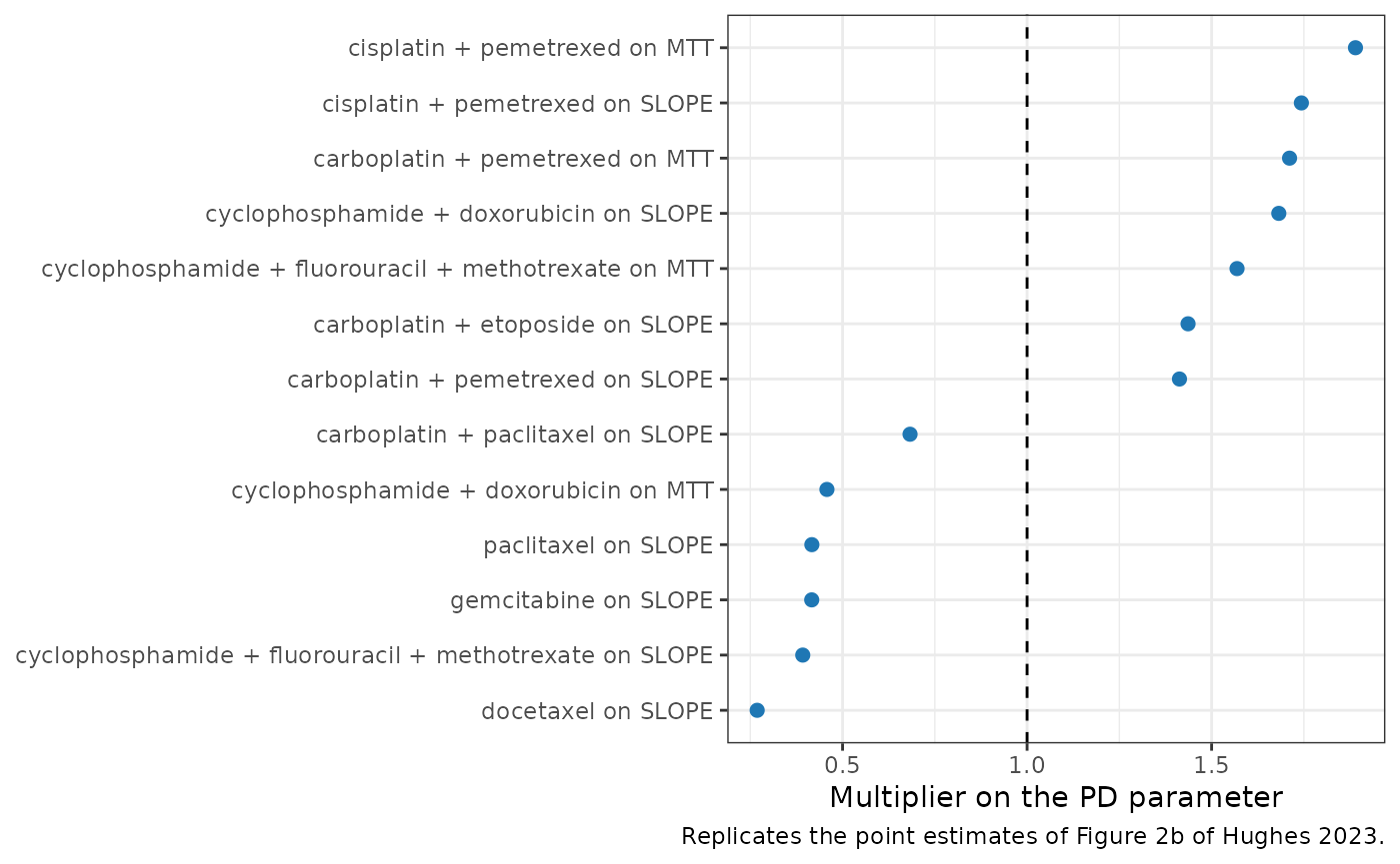
Typical-value profiles
All five neutrophil compartments start at CIRC0. With no drug, the chain must stay exactly at baseline, and a baseline ANC below 0.5 x 10^9/L must be raised to 0.5.
trt_cols <- c(
  "TRT_CYCLOPHOSPHAMIDE_DOXORUBICIN", "TRT_CARBOPLATIN_ETOPOSIDE",
  "TRT_CARBOPLATIN_PACLITAXEL", "TRT_CARBOPLATIN_PEMETREXED",
  "TRT_CISPLATIN_PEMETREXED", "TRT_CYCLOPHOSPHAMIDE_FLUOROURACIL_METHOTREXATE",
  "TRT_DOCETAXEL", "TRT_GEMCITABINE", "TRT_PACLITAXEL"
)

# One subject: three 21-day cycles of a population-average chemotherapy dose
# (amount 1), optional G-CSF one day after each chemotherapy dose, and daily
# ANC observations on the circulating-neutrophil state.
make_subject <- function(id, regimen = "reference", gcsf = "none",
                         neut = 4.8, age = 57.2, alb = 41, chemo = TRUE) {
  cyc <- c(0, 504, 1008)
  dose <- if (chemo) {
    tibble(time = cyc, evid = 1L, amt = 1, cmt = "depot_kpd")
  } else {
    tibble(time = numeric(0), evid = integer(0), amt = numeric(0), cmt = character(0))
  }
  if (gcsf != "none") {
    dose <- bind_rows(dose, tibble(time = cyc + 24, evid = 1L, amt = 1, cmt = "depot"))
  }
  obs <- tibble(time = seq(0, 1512, by = 6), evid = 0L, amt = 0, cmt = "circ")
  ev <- bind_rows(dose, obs) |>
    arrange(time, desc(evid)) |>
    mutate(
      id = id, regimen = regimen, gcsf = gcsf,
      NEUT = neut, AGE = age, ALB = alb,
      FORM_GCSF_PEG = as.integer(gcsf == "pegfilgrastim")
    )
  for (tc in trt_cols) ev[[tc]] <- as.integer(regimen == tc)
  ev
}

mod_typ <- rxode2::zeroRe(mod)
#> ℹ parameter labels from comments will be replaced by 'label()'
ev_ss <- bind_rows(
  make_subject(1, chemo = FALSE, neut = 4.8),
  make_subject(2, chemo = FALSE, neut = 0.3)
)
sim_ss <- rxode2::rxSolve(mod_typ, events = ev_ss, keep = "NEUT") |>
  as.data.frame()
#> ℹ omega/sigma items treated as zero: 'etalslope', 'etalmtt', 'etalstm1', 'etalcirc0'
#> Warning: multi-subject simulation without without 'omega'
ss <- sim_ss |>
  group_by(id, NEUT) |>
  summarise(min_anc = min(ANC), max_anc = max(ANC), .groups = "drop")
knitr::kable(ss, digits = 6, caption = "No-drug steady state (expected: max(NEUT, 0.5)).")| id | NEUT | min_anc | max_anc |
|---|---|---|---|
| 1 | 4.8 | 4.8 | 4.8 |
| 2 | 0.3 | 0.5 | 0.5 |
stopifnot(
  all(abs(ss$min_anc - pmax(ss$NEUT, 0.5)) < 1e-6),
  all(abs(ss$max_anc - pmax(ss$NEUT, 0.5)) < 1e-6)
)
The paper does not tabulate typical-value nadirs. The profiles below show how each regimen group, and G-CSF for the reference group, changes the cycle-1 nadir of a typical patient (age 57.2 years, albumin 4.1 g/dL, baseline ANC 4.8 x 10^9/L).
scen <- tibble(regimen = c("reference", trt_cols), gcsf = "none") |>
  bind_rows(tibble(regimen = "reference", gcsf = c("filgrastim", "pegfilgrastim")))
ev_typ <- bind_rows(lapply(seq_len(nrow(scen)), function(i) {
  make_subject(i, regimen = scen$regimen[i], gcsf = scen$gcsf[i])
}))
sim_typ <- rxode2::rxSolve(mod_typ, events = ev_typ, keep = c("regimen", "gcsf")) |>
  as.data.frame()
#> ℹ omega/sigma items treated as zero: 'etalslope', 'etalmtt', 'etalstm1', 'etalcirc0'
#> Warning: multi-subject simulation without without 'omega'

nadir_tab <- sim_typ |>
  filter(time < 504) |>
  group_by(regimen, gcsf) |>
  summarise(
    nadir = min(ANC),
    day_nadir = time[which.min(ANC)] / 24,
    .groups = "drop"
  ) |>
  mutate(regimen = sub("^TRT_", "", regimen)) |>
  arrange(nadir)
nadir_tab |>
  dplyr::rename(
    "Regimen group" = regimen, "G-CSF" = gcsf,
    "Cycle-1 nadir (10^9/L)" = nadir, "Day of nadir" = day_nadir
  ) |>
knitr::kable(digits = 2, caption = "Typical-value cycle-1 ANC nadir by regimen group.")| Regimen group | G-CSF | Cycle-1 nadir (10^9/L) | Day of nadir |
|---|---|---|---|
| CYCLOPHOSPHAMIDE_DOXORUBICIN | none | 0.72 | 5.25 |
| CARBOPLATIN_ETOPOSIDE | none | 2.21 | 10.00 |
| reference | none | 2.79 | 9.75 |
| reference | filgrastim | 2.84 | 9.75 |
| reference | pegfilgrastim | 2.89 | 9.50 |
| CISPLATIN_PEMETREXED | none | 2.90 | 18.00 |
| CARBOPLATIN_PEMETREXED | none | 3.06 | 16.25 |
| CARBOPLATIN_PACLITAXEL | none | 3.31 | 9.75 |
| PACLITAXEL | none | 3.82 | 9.50 |
| GEMCITABINE | none | 3.82 | 9.50 |
| DOCETAXEL | none | 4.14 | 9.50 |
| CYCLOPHOSPHAMIDE_FLUOROURACIL_METHOTREXATE | none | 4.18 | 14.75 |
ref_nadir <- nadir_tab |> filter(regimen == "reference", gcsf == "none")
peg_nadir <- nadir_tab |> filter(regimen == "reference", gcsf == "pegfilgrastim")
fil_nadir <- nadir_tab |> filter(regimen == "reference", gcsf == "filgrastim")
stopifnot(
  nrow(ref_nadir) == 1, nrow(peg_nadir) == 1, nrow(fil_nadir) == 1,
  # The Figure S2b observed median falls from about 5 to about 3 x 10^9/L
  # (ratio ~0.6) around day 8; the typical reference-regimen patient gives 0.58.
  ref_nadir$nadir / 4.8 > 0.45, ref_nadir$nadir / 4.8 < 0.75,
  ref_nadir$day_nadir > 7, ref_nadir$day_nadir < 12,
  # Deterministic (no random effects): G-CSF raises the nadir.
  peg_nadir$nadir > ref_nadir$nadir,
  fil_nadir$nadir > ref_nadir$nadir
)

sim_typ |>
  filter(gcsf == "none") |>
  mutate(regimen = sub("^TRT_", "", regimen)) |>
  ggplot(aes(time / 24, ANC, colour = regimen)) +
  geom_line() +
  geom_hline(yintercept = 1, linetype = "dotted") +
  scale_y_log10() +
  labs(
    x = "Time (days)", y = "ANC (10^9/L)", colour = "Regimen group",
    caption = "Typical patient, population-average dose (amount 1) every 21 days."
  ) +
  theme_bw() +
  theme(legend.position = "bottom", legend.text = element_text(size = 6))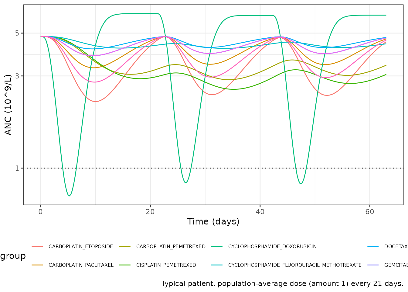
The G-CSF effect per population-average dose is small: one dose of filgrastim or pegfilgrastim raises the typical cycle-1 nadir by a few percent. The paper also reports muted peaks and nadirs in individual predictions (Results, “Model performance”). It suggests that the effects of G-CSF and of strongly neutropenic regimens such as docetaxel were not separately identifiable, because prophylactic G-CSF is usually prescribed with those regimens (Discussion).
Visual predictive check (Figure S2b)
Figure S2b compares the 5th, 50th and 95th percentiles of observed ANC with simulated data against time after cycle start. The observed patients’ regimen mix is not published, so the virtual cohort below draws each patient’s regimen group with equal probability from the nine groups and the reference group. It also draws age and albumin around the Table 1 medians. Baseline ANC is drawn log-normally around the Table 1 median ANC of 4.8 x 10^9/L.
set.seed(2023)
rxode2::rxSetSeed(2023)
n_vpc <- 200
cohort <- tibble(
  id = seq_len(n_vpc),
  AGE = pmin(pmax(rnorm(n_vpc, 57.7, 12), 20), 89),
  ALB = pmin(pmax(rnorm(n_vpc, 42, 4), 17), 53),
  NEUT = exp(rnorm(n_vpc, log(4.8), 0.35)),
  FORM_GCSF_PEG = 0L,
  regimen = sample(c("reference", trt_cols), n_vpc, replace = TRUE)
)
for (tc in trt_cols) cohort[[tc]] <- as.integer(cohort$regimen == tc)

ev_vpc <- bind_rows(
  tidyr::expand_grid(id = cohort$id, time = c(0, 504, 1008)) |>
    mutate(evid = 1L, amt = 1, cmt = "depot_kpd"),
  tidyr::expand_grid(id = cohort$id, time = seq(0, 1512, by = 24)) |>
    mutate(evid = 0L, amt = 0, cmt = "circ")
) |>
  left_join(cohort, by = "id") |>
  arrange(id, time, desc(evid))
stopifnot(!anyDuplicated(unique(ev_vpc[, c("id", "time", "evid")])))

sim_vpc <- rxode2::rxSolve(mod, events = ev_vpc, keep = "regimen") |>
  as.data.frame()
#> ℹ parameter labels from comments will be replaced by 'label()'
vpc <- sim_vpc |>
  mutate(day = (time %% 504) / 24) |>
  group_by(day) |>
  summarise(
    p05 = quantile(sim, 0.05),
    p50 = quantile(sim, 0.50),
    p95 = quantile(sim, 0.95),
    .groups = "drop"
  )

ggplot(vpc, aes(day)) +
  geom_ribbon(aes(ymin = p05, ymax = p95), fill = "#1f77b4", alpha = 0.2) +
  geom_line(aes(y = p50), linewidth = 1) +
  geom_line(aes(y = p05), linetype = "dashed") +
  geom_line(aes(y = p95), linetype = "dashed") +
  scale_y_log10(breaks = c(0.3, 1, 3, 10, 30)) +
  labs(
    x = "Time after cycle start (days)", y = "ANC (k/uL)",
    caption = paste(
      "Simulated 5th, 50th and 95th percentiles (with residual error), three",
      "21-day cycles pooled. Compare with Figure S2b of Hughes 2023."
    )
  ) +
  theme_bw()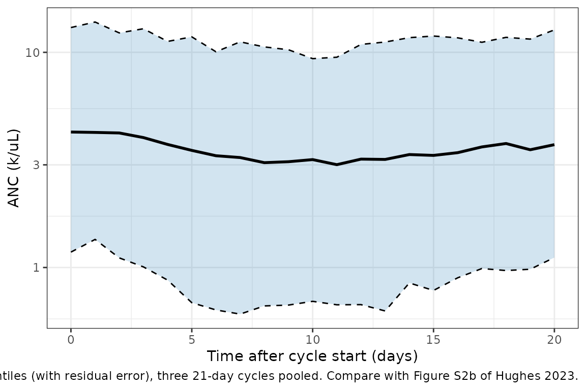
# Centre of the distribution only (robust to which subjects land in the tails).
# Figure S2b: observed median about 5 at cycle start and about 3 at days 7-10.
med_start <- vpc$p50[vpc$day == 0]
med_nadir <- min(vpc$p50[vpc$day >= 6 & vpc$day <= 12])
stopifnot(
  length(med_start) == 1,
  med_start > 3, med_start < 7,
  med_nadir > 2, med_nadir < 4.5,
  med_nadir < med_start
)
The simulated median falls from about 4.3 to about 3 x 10^9/L between days 6 and 12, close to the observed median in Figure S2b (about 5 falling to about 3 around day 8). The observed 5th percentile falls lower (about 0.4 x 10^9/L near day 8) than the simulated one. The virtual cohort gives no G-CSF and spreads patients evenly over the regimen groups, so it is a qualitative check of the model’s shape, not a reconstruction of the test set.
G-CSF pharmacokinetics (PKNCA)
The control stream states that the fixed G-CSF clearance was chosen to give the Melhem 2018 half-lives: 2.6 h for filgrastim and 10.1 h for pegfilgrastim, with V = 50 L. After a subcutaneous dose the terminal phase is absorption-limited (flip-flop): the absorption half-life is 5.6 h for filgrastim and 36.9 h for pegfilgrastim. The elimination half-life is therefore checked with PKNCA on a bolus placed directly into the G-CSF central compartment.
ev_pk <- bind_rows(lapply(c(filgrastim = 0L, pegfilgrastim = 1L), function(peg) {
  bind_rows(
    tibble(time = 0, evid = 1L, amt = 1, cmt = "central"),
    tibble(time = c(0, seq(0.25, 120, by = 0.25)), evid = 0L, amt = 0, cmt = "central")
  ) |>
    mutate(
      id = peg + 1L, FORM_GCSF_PEG = peg,
      treatment = ifelse(peg == 1L, "pegfilgrastim", "filgrastim")
    )
})) |>
  mutate(NEUT = 4.8, AGE = 57.2, ALB = 41)
for (tc in trt_cols) ev_pk[[tc]] <- 0L

sim_pk <- rxode2::rxSolve(
  mod_typ,
  events = ev_pk, keep = "treatment", rtol = 1e-10, atol = 1e-12
) |>
  as.data.frame() |>
  mutate(Cc = central / 50)
#> ℹ omega/sigma items treated as zero: 'etalslope', 'etalmtt', 'etalstm1', 'etalcirc0'
#> Warning: multi-subject simulation without without 'omega'

conc_pk <- sim_pk |>
  filter(!is.na(Cc)) |>
  select(id, treatment, time, Cc) |>
  distinct(id, treatment, time, .keep_all = TRUE)
dose_pk <- ev_pk |>
  filter(evid == 1) |>
  select(id, treatment, time, amt)

nca_pk <- PKNCA::pk.nca(PKNCA::PKNCAdata(
  PKNCA::PKNCAconc(conc_pk, Cc ~ time | treatment + id),
  PKNCA::PKNCAdose(dose_pk, amt ~ time | treatment + id, route = "intravascular"),
  intervals = data.frame(start = 0, end = Inf, half.life = TRUE)
))

published_pk <- tibble::tribble(
  ~treatment, ~half.life,
  "filgrastim", 2.6,
  "pegfilgrastim", 10.1
)
pk_cmp <- nlmixr2lib::ncaComparisonTable(
  simulated = nca_pk,
  reference = published_pk,
  by = "treatment",
  units = c(half.life = "h"),
  tolerance_pct = 20
)
knitr::kable(
  pk_cmp,
  caption = paste(
    "G-CSF elimination half-life, simulated (PKNCA) vs. the Appendix S2",
    "control-stream comment. * differs by >20%."
  )
)| NCA parameter | treatment | Reference | Simulated | % diff |
|---|---|---|---|---|
| t½ (h) | filgrastim | 2.6 | 2.61 | +0.2% |
| t½ (h) | pegfilgrastim | 10.1 | 10.1 | +0.0% |
Assumptions and deviations
- XGBoost layer not included. The ML, enriched and augmented models of the paper are tree ensembles trained on non-public data. Only their PKPD backbone, which is fully specified in Appendix S2, is shipped.
- Dose units are normalized. The paper normalized every dose to the training-population average dose of that drug after BSA scaling, but does not report those average doses. Users therefore supply normalized amounts (1 = population-average dose). The paper states this normalization for “each dose for each medication”. The maintainers applied it to G-CSF as well, because ST1 and ST2 act on the G-CSF central amount: an amount in micrograms would make proliferation grow several thousand-fold after one dose.
-
Chemotherapy is a K-PD state. The control stream
names compartment 1 “CENTR”, but the data contained no drug
concentrations and CL and V are fixed (Results, “PKPD model
development”), so the state is encoded as the registered
depot_kpd. Its elimination rate iskel = CLchemo / V = 0.1 1/h. -
Regimen indicators. The NONMEM
REGcode is replaced by nine mutually exclusiveTRT_<regimen>indicators, one per estimated regimen group. Each indicator covers the cytotoxic backbone with or without monoclonal antibodies or immunotherapy, following the regimen-to-THETA mapping of Appendix S2 (the full code lists are in the model’scovariateDatanotes). Regimens whose THETA was fixed to 1, regimens given to fewer than 50 training patients, and any regimen not listed take all indicators at 0. -
Baseline random effect. NONMEM writes CIRC0 as
CIRCBL * exp(ETA(3) * sqrt(SIGMA))withOMEGA(3) = 1 FIX, so the baseline eta has the residual variance (Dansirikul method). The model encodes it asetalcirc0 ~ fixed(0.162848), which gives the same distribution. If the residual variance is re-estimated,etalcirc0must be updated to match it by hand. -
Residual error.
Y = LOG(IPRED + 0.00001) + EPS(1)is encoded aslnorm(expSd). The 1e-5 offset only matters at ANC values far below the data range and is omitted. -
Covariate units. Serum albumin is supplied in g/L
(the canonical column) and converted to g/dL inside the model. Baseline
ANC (
NEUT) is supplied in 10^9/L, the paper’s unit. - Virtual cohort. The regimen mix, the baseline ANC spread (log-SD 0.35) and the absence of G-CSF in the VPC cohort are assumptions. Table 1 reports only cancer type, G-CSF use and summary demographics.
- No erratum or correction notice was found for this article as of 2026-10-28.