Varenicline (Ravva 2009)
Source:vignettes/articles/Ravva_2009_varenicline.Rmd
Ravva_2009_varenicline.RmdModel and source
- Citation: Ravva P, Gastonguay MR, Tensfeldt TG, Faessel HM. Population pharmacokinetic analysis of varenicline in adult smokers. Br J Clin Pharmacol. 2009;68(5):669-681. doi:10.1111/j.1365-2125.2009.03520.x
- Description: Two-compartment population PK model with first-order absorption and lag-time for varenicline in adult smokers (Ravva 2009): apparent clearance scales with creatinine clearance and race; central volume scales with body weight, age, and race; peripheral disposition uses fixed allometric exponents on weight.
- Article: https://doi.org/10.1111/j.1365-2125.2009.03520.x
Ravva and colleagues developed a two-compartment population PK model with first-order absorption and a lag time for varenicline tartrate (Pfizer Chantix / Champix) in adult smokers. The structural model and covariate relationships in Table 4 of the source paper are reproduced verbatim, with the volunteer-study (Studies I) residual-error magnitudes encoded as the primary error model; see the Assumptions and deviations section for the alternative patient-study (Studies II + III) residual-error values.
Population
The model was fit to pooled plasma varenicline data from nine clinical trials in 1878 adult smokers (954 male, 924 female): four phase-I volunteer studies (N = 198), two phase-II trials (N = 858), and three phase-III trials (N = 822) with sampling windows ranging from 7 days to 52 weeks. Doses were administered orally as immediate-release tablets at 0.3 to 3 mg/day, once-daily or twice-daily. Baseline demographics (Ravva 2009 Table 2): mean age 44.0 years (range 18 to 76), mean body weight 78.0 kg (range 41 to 129), height range 135 to 202 cm, BMI range 16.0 to 44.8 kg/m^2, and Cockcroft-Gault estimated creatinine clearance with mean 112 mL/min (range 15.6 to 268, truncated at the upper value 150 mL/min). About 15 percent of subjects had mild-to-severe renal impairment. Race distribution: White 81.0 percent, Black 12.6 percent, Asian 1.22 percent, Other 5.22 percent. The total dataset contains 11 935 quantifiable plasma concentrations after removal of 664 (4 percent) BLQ records (Methods).
The same information is available programmatically via the model’s
population metadata
(readModelDb("Ravva_2009_varenicline")$population).
Source trace
The per-parameter origin is recorded as an in-file comment next to
each ini() entry in
inst/modeldb/specificDrugs/Ravva_2009_varenicline.R. The
table below collects them in one place for review.
| Equation / parameter | Value | Source location |
|---|---|---|
lka |
log(1.69) | Table 4 (Ka) |
lcl |
log(10.4) | Table 4 (q_CL); typical CL/F at White, 70 kg, 45 y, CLcr=100 mL/min |
lvc |
log(337) | Table 4 (q_V2) |
lvp |
log(78.1) | Table 4 (q_V3) |
lq |
log(2.08) | Table 4 (q_Q) |
ltlag |
log(0.43) | Table 4 (q_Alag) |
e_crcl_cl |
0.54 | Table 4 (q_CRCL on CL/F); power-form, reference 100 mL/min (Discussion) |
e_black_cl |
1.16 | Table 4 (q_Black on CL/F); power-of-indicator form |
e_other_cl |
1.11 | Table 4 (q_Other on CL/F); power-of-indicator form |
e_wt_vc |
0.77 | Table 4 (q_WT on V2/F); power-form, reference 70 kg |
e_age_vc |
0.13 | Table 4 (q_AGE on V2/F); power-form, reference 45 years |
e_black_vc |
0.92 | Table 4 (q_Black on V2/F); power-of-indicator form |
e_other_vc |
0.71 | Table 4 (q_Other on V2/F); power-of-indicator form |
e_wt_vp |
1 (Fixed) | Table 4 (q_WT on V3/F); allometric exponent held fixed |
e_wt_q |
0.75 (Fixed) | Table 4 (q_WT on Q/F); allometric exponent held fixed |
| IIV block (Ka, CL, V2) | var 0.49, 0.061, 0.25; cov 0.24, 0.006, -0.009 | Table 4 (Interindividual variance block); reported %CV = 70.1, 24.7, 50.0 |
addSd |
0.5 (= sqrt(0.28)) | Table 4 (s^2_add,1) for volunteer Studies I |
propSd |
0.172 (= sqrt(0.030)) | Table 4 (s^2_prop,1) for volunteer Studies I |
| Two-compartment structure with first-order absorption and lag | n/a | Methods (ADVAN4/TRANS4) and Results paragraph on final structural model |
The Studies II + III (large patient trials) error magnitudes –
addSd_pat = 2.1 (s^2_add,2 = 4.38) and
propSd_pat = 0.215 (s^2_prop,2 = 0.046) – are NOT encoded
in the packaged model. See Assumptions and deviations for the
rationale.
Virtual cohort
Original observed data are not publicly available. The virtual cohort below mirrors the typical-individual covariate set used in Ravva 2009 (White, 70 kg, 45 years, CLcr = 100 mL/min) and a renal-function stratification at 0.5 mg q.d. matching the cohort cut-offs Ravva 2009 uses in the Discussion.
set.seed(20260613)

# Helper: build a single-cohort event table with covariates already attached.
# `id_offset` lets us stack cohorts via bind_rows() without collisions.
make_cohort <- function(n, ka_dose_mg, dose_interval_h, n_doses,
                        wt, age, crcl,
                        race_black = 0, race_other = 0,
                        treatment_label, id_offset = 0L) {
  ids <- id_offset + seq_len(n)
  obs_grid <- seq(0, dose_interval_h * (n_doses + 2), by = 0.5)
  obs <- expand.grid(id = ids, time = obs_grid)
  obs$evid <- 0L
  obs$amt  <- 0
  obs$cmt  <- "central"
  dose_times <- (0:(n_doses - 1)) * dose_interval_h
  dos <- expand.grid(id = ids, time = dose_times)
  dos$evid <- 1L
  dos$amt  <- ka_dose_mg
  dos$cmt  <- "depot"
  ev <- dplyr::bind_rows(obs, dos)
  ev$WT         <- wt
  ev$AGE        <- age
  ev$CRCL       <- crcl
  ev$RACE_BLACK <- race_black
  ev$RACE_OTHER <- race_other
  ev$treatment  <- treatment_label
  ev[order(ev$id, ev$time, -ev$evid), ]
}

# Cohort A: typical White subject, 1 mg b.i.d., 10 days to steady state.
events_a <- make_cohort(
  n = 100L, ka_dose_mg = 1, dose_interval_h = 12, n_doses = 20,
  wt = 70, age = 45, crcl = 100,
  treatment_label = "1 mg b.i.d. (typical, CLcr 100)",
  id_offset = 0L
)

# Cohorts B-E: renal-function stratification at 0.5 mg q.d. for 10 doses.
events_b <- make_cohort(80L, 0.5, 24, 10, 70, 45, 100,
                        treatment_label = "0.5 mg q.d. (CLcr 100)",
                        id_offset = 100L)
events_c <- make_cohort(80L, 0.5, 24, 10, 70, 45, 65,
                        treatment_label = "0.5 mg q.d. (CLcr 65, mild RI)",
                        id_offset = 200L)
events_d <- make_cohort(80L, 0.5, 24, 10, 70, 45, 40,
                        treatment_label = "0.5 mg q.d. (CLcr 40, moderate RI)",
                        id_offset = 300L)
events_e <- make_cohort(80L, 0.5, 24, 10, 70, 45, 20,
                        treatment_label = "0.5 mg q.d. (CLcr 20, severe RI)",
                        id_offset = 400L)

events <- dplyr::bind_rows(events_a, events_b, events_c, events_d, events_e)
stopifnot(!anyDuplicated(unique(events[, c("id", "time", "evid")])))
Simulation
mod <- readModelDb("Ravva_2009_varenicline")

# Typical-value simulation (no BSV, no residual error) reproduces the paper's
# published steady-state typical-individual exposures.
mod_typical <- rxode2::zeroRe(mod)
sim_typical <- rxode2::rxSolve(mod_typical, events = events,
                               keep = c("treatment"))
#> ℹ omega/sigma items treated as zero: 'etalka', 'etalcl', 'etalvc'
#> Warning: multi-subject simulation without without 'omega'
sim_typical <- as.data.frame(sim_typical)
Replicate published exposures
# Replicates Ravva 2009 Discussion: typical 1 mg b.i.d. steady-state profile
# (paper reports AUC0-24,ss = 186 ng*h/mL and Cavg,ss = 7.73 ng/mL).
sim_typical |>
  dplyr::filter(treatment == "1 mg b.i.d. (typical, CLcr 100)",
                id == min(id),
                time >= 168, time <= 192) |>
  ggplot(aes(time - 168, Cc)) +
  geom_line() +
  labs(x = "Time within steady-state dosing interval (h)",
       y = "Plasma varenicline (ng/mL)",
       title = "Typical steady-state profile at 1 mg b.i.d.",
       caption = "Reproduces Ravva 2009 Discussion typical-individual exposures.")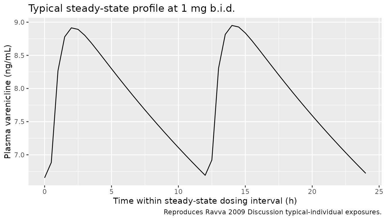
# Replicates Ravva 2009 Figure 8 + Discussion: typical 0.5 mg q.d. profiles
# stratified by renal function. CL/F decreases progressively from 10.4 L/h
# (CLcr=100) to 4.4 L/h (CLcr=20), increasing varenicline exposure by ~2.4-fold
# at severe RI relative to normal renal function.
sim_typical |>
  dplyr::filter(grepl("0.5 mg q.d.", treatment),
                id %in% c(101, 201, 301, 401),
                time >= 192, time <= 240) |>
  dplyr::mutate(time_in_interval = time - 192) |>
  ggplot(aes(time_in_interval, Cc, colour = treatment)) +
  geom_line() +
  labs(x = "Time within steady-state dosing interval (h)",
       y = "Plasma varenicline (ng/mL)",
       colour = "Renal function",
       title = "Typical steady-state profile at 0.5 mg q.d. by renal function",
       caption = "Reproduces Ravva 2009 Discussion exposure-by-renal-function summary.")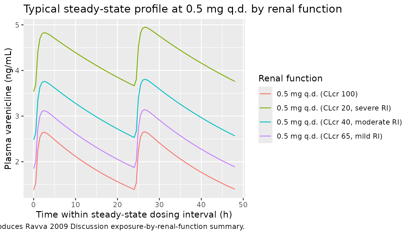
PKNCA validation
# 1 mg b.i.d. cohort -- compute NCA on the last steady-state dosing interval
# (time 228 to 240 hours after the first dose), which lies within the
# observation window of all 100 subjects.
sim_nca_bid <- sim_typical |>
  dplyr::filter(treatment == "1 mg b.i.d. (typical, CLcr 100)",
                time >= 228, time <= 240) |>
  dplyr::mutate(time = time - 228) |>
  dplyr::filter(!is.na(Cc)) |>
  dplyr::select(id, time, Cc, treatment)

# Ensure a t = 0 record per (id, treatment) for the AUC anchor.
sim_nca_bid <- dplyr::bind_rows(
  sim_nca_bid,
  sim_nca_bid |> dplyr::distinct(id, treatment) |>
    dplyr::mutate(time = 0, Cc = min(sim_nca_bid$Cc[sim_nca_bid$time == 0]))
) |>
  dplyr::distinct(id, treatment, time, .keep_all = TRUE) |>
  dplyr::arrange(id, treatment, time)

# Build a representative SS dosing record at time 0 of the synthetic window.
dose_bid <- sim_nca_bid |> dplyr::distinct(id, treatment) |>
  dplyr::mutate(time = 0, amt = 1)

conc_obj_bid <- PKNCA::PKNCAconc(sim_nca_bid, Cc ~ time | treatment + id,
                                 concu = "ng/mL", timeu = "h")
dose_obj_bid <- PKNCA::PKNCAdose(dose_bid, amt ~ time | treatment + id,
                                 doseu = "mg")

intervals_bid <- data.frame(
  start   = 0,
  end     = 12,
  cmax    = TRUE,
  tmax    = TRUE,
  cmin    = TRUE,
  auclast = TRUE,
  cav     = TRUE
)
nca_bid <- PKNCA::pk.nca(PKNCA::PKNCAdata(conc_obj_bid, dose_obj_bid,
                                         intervals = intervals_bid))

# Compute AUC0-24 from two consecutive 12-h intervals (paper reports AUC0-24,ss).
auclast_bid <- as.data.frame(nca_bid$result) |>
  dplyr::filter(PPTESTCD == "auclast") |>
  dplyr::pull(PPORRES)
auc0_24_bid <- mean(auclast_bid) * 2  # two 12-h intervals make one 24-h interval at SS
cav_bid <- as.data.frame(nca_bid$result) |>
  dplyr::filter(PPTESTCD == "cav") |>
  dplyr::pull(PPORRES)
Comparison against published NCA
The paper reports overall steady-state mean values at 1 mg b.i.d. (Discussion): AUC0-24,ss = 186 ng*h/mL, Cavg,ss = 7.73 ng/mL. The simulated typical-individual values are compared below.
published <- tibble::tribble(
  ~treatment,                              ~auclast, ~cav,
  "1 mg b.i.d. (typical, CLcr 100)",       93.0,     7.73
)
# AUC over the 12-h dosing interval at SS = 186 / 2 = 93 ng*h/mL.

cmp <- nlmixr2lib::ncaComparisonTable(
  simulated     = nca_bid,
  reference     = published,
  by            = "treatment",
  units         = c(auclast = "ng*h/mL", cav = "ng/mL"),
  tolerance_pct = 20
)

knitr::kable(
  cmp,
  caption = "Simulated vs. published steady-state NCA at 1 mg b.i.d. AUC is over the 12-h dosing interval; the paper's reported AUC0-24,ss = 186 ng*h/mL halves to 93 ng*h/mL per 12-h interval at steady state. * differs from reference by >20%.",
  align   = c("l", "l", "l", "r", "r", "r")
)| NCA parameter | treatment | Reference | Simulated | % diff |
|---|---|---|---|---|
| AUClast (ng*h/mL) | 1 mg b.i.d. (typical, CLcr 100) | 93 | 95.4 | +2.6% |
| Cavg (ng/mL) | 1 mg b.i.d. (typical, CLcr 100) | 7.73 | 7.95 | +2.9% |
Renal-function CL/F replication
Ravva 2009 (Discussion) reports the typical CL/F decreases
progressively with declining renal function: 10.4 L/h at CLcr = 100
(normal), 8.3 L/h at CLcr = 65 (mild RI), 6.4 L/h at CLcr = 40 (moderate
RI), and 4.4 L/h at CLcr = 20 (severe RI). The model’s analytic
prediction is CL = exp(lcl) * (CRCL/100)^e_crcl_cl for a
White subject; the table below recomputes these values and compares to
the paper.
mod_obj  <- mod()
mod_ini  <- as.data.frame(mod_obj$ini)
theta    <- setNames(mod_ini$est, mod_ini$name)
cl_typical <- function(crcl) exp(theta[["lcl"]]) * (crcl / 100)^theta[["e_crcl_cl"]]

renal_cmp <- tibble::tibble(
  Cohort       = c("Normal (CLcr=100)", "Mild RI (CLcr=65)",
                   "Moderate RI (CLcr=40)", "Severe RI (CLcr=20)"),
  CLcr_mL_min  = c(100, 65, 40, 20),
  CL_paper     = c(10.4, 8.3, 6.4, 4.4),
  CL_model     = round(c(cl_typical(100), cl_typical(65),
                         cl_typical(40), cl_typical(20)), 2)
)
renal_cmp$pct_diff <- round(100 * (renal_cmp$CL_model - renal_cmp$CL_paper) /
                                  renal_cmp$CL_paper, 1)
knitr::kable(
  renal_cmp,
  caption = "Typical CL/F by renal function (L/h). Paper values from Ravva 2009 Discussion; model values from `exp(lcl) * (CRCL / 100)^e_crcl_cl` evaluated at the population-typical reference CLcr.",
  align   = c("l", "r", "r", "r", "r")
)| Cohort | CLcr_mL_min | CL_paper | CL_model | pct_diff |
|---|---|---|---|---|
| Normal (CLcr=100) | 100 | 10.4 | 10.40 | 0.0 |
| Mild RI (CLcr=65) | 65 | 8.3 | 8.24 | -0.7 |
| Moderate RI (CLcr=40) | 40 | 6.4 | 6.34 | -0.9 |
| Severe RI (CLcr=20) | 20 | 4.4 | 4.36 | -0.9 |
Assumptions and deviations
Residual error: volunteer studies only. Ravva 2009 Table 4 reports two distinct residual-error structures: one for the four small phase-I volunteer studies (intensive sampling, controlled timing) with s^2_add,1 = 0.28 (SD = 0.5 ng/mL) and s^2_prop,1 = 0.030 (17.2 percent CV), and a second, larger structure for the five large phase-II / phase-III patient trials (sparse sampling, outpatient timing) with s^2_add,2 = 4.38 (SD = 2.1 ng/mL) and s^2_prop,2 = 0.046 (21.5 percent CV). The volunteer (Studies I) values characterize the intrinsic PK + bioanalytical-assay noise; the patient (Studies II + III) values include additional operational noise from sparse sampling and outpatient dose timing. The packaged model encodes the volunteer values as the primary
addSdandpropSd. To simulate the patient-trial residual-error magnitude instead, replace the values inini()with the Studies II + III magnitudes given here. Both error structures share the same structural model and parameter set; only the residual-error magnitudes differ.Race / ethnicity composite “Other”. Ravva 2009 groups Hispanic + Asian + Other into one composite category for the race covariate effect on CL/F and V2/F because the individual subgroups were each less than 5 percent of the population. The packaged model uses the canonical
RACE_OTHERindicator for this composite. Users simulating cohorts with a meaningfully large Asian or Hispanic subgroup should be aware that the model does not separate them.Cockcroft-Gault CRCL is raw, not BSA-normalized. The canonical CRCL column in
inst/references/covariate-columns.mdis defined as BSA-normalized mL/min/1.73 m^2, but Ravva 2009 used raw Cockcroft-Gault estimated CrCl in mL/min and normalized to a reference of 100 mL/min. The packaged model follows the Ravva 2009 convention with reference 100 mL/min raw, matching the precedent set byDelattre_2010_amikacin.R(which also uses raw Cockcroft-Gault mL/min for CRCL).CRCL truncation at 150 mL/min. Ravva 2009 truncated estimated CrCl values at an upper bound of 150 mL/min (Results) to drop physiologically improbable Cockcroft-Gault upper-tail values. Users simulating cohorts with CRCL > 150 mL/min should clamp at 150 to match the model’s estimation range.
No reference IV data. Varenicline does not have published IV PK, so all parameters are apparent (
CL/F,V2/F, etc.). The packaged model cannot separately estimate absolute bioavailability F; only the dose * F composite that determines plasma exposure.AGE effect on V2/F was poorly defined. Ravva 2009 reports the AGE exponent on V2/F as 0.13 with 54.1 percent RSE and a 95 percent CI that includes zero. The exponent is encoded faithfully but should be viewed as exploratory; users simulating ages outside 18 to 76 should treat the AGE contribution to V2/F with caution.