Nortriptyline (Vos 2025)
Source:vignettes/articles/Vos_2025_nortriptyline.Rmd
Vos_2025_nortriptyline.RmdModel and source
- Citation: Vos CF, Coenen MJH, ter Hark SE, Schellekens AFA, Aarnoutse RE, Janzing JGE, ter Heine R. Optimizing Nortriptyline Dosing: A Comparison between Pharmacogenetics-Based, Phenotype-Based, and Standard Dosing. Clin Pharmacokinet. 2025;64(7):1071-1078. doi:10.1007/s40262-025-01528-x
- Description: One-compartment population PK model for oral nortriptyline in adults with major depressive disorder (Vos 2025): first-order absorption with the rate constant fixed from Kvist 2001, and a well-stirred liver in which the intrinsic clearance CLint (with interindividual variability) sets both the systemic clearance Q * CLint / (Q + CLint) and the hepatic availability Q / (Q + CLint), with hepatic plasma flow Q fixed to 36 L/h.
- Article: Clin Pharmacokinet 2025;64(7):1071-1078
- Supplement: Electronic Supplementary Material 1 (ESM 1) of the article, which holds the model equations and the parameter table.
Vos et al. developed this model to turn one nortriptyline plasma
concentration measured 8-24 h after the first dose into a steady-state
dose recommendation (“phenotype-based dosing”). They then compared that
strategy with CYP2D6 genotype-guided dosing and with a fixed 125 mg/day
dose. The structural model follows “model 2” of Kvist et al. (Clin
Pharmacokinet 2001;40:869-877). Oral nortriptyline is absorbed
first-order into a single central compartment. A well-stirred liver
links clearance and bioavailability: the intrinsic clearance CLint, the
only parameter with interindividual variability, sets both the systemic
clearance CL = Q * CLint / (Q + CLint) and the hepatic
availability F = Q / (Q + CLint). The apparent oral
clearance CL / F therefore equals CLint, and
the average steady-state concentration is simply
dose rate / CLint.
Population
The model was fitted to 85 adults (18-65 years) with major depressive disorder who were treated with nortriptyline in the Dutch PITA randomized controlled trial and had at least one measured plasma concentration (Methods; ESM 1). Participants were free of other psychotropic medication, apart from benzodiazepines up to 4 mg lorazepam-equivalent per day, and of interacting co-medication. The article reports demographics only for the 48 participants used in the dosing-strategy comparison (Table 1): 48% female, mean age 42.0 (SD 13.8) years, and CYP2D6 genotype-predicted phenotypes of 5 poor (PM), 20 intermediate (IM), 21 normal (NM) and 2 ultra-rapid (UM) metabolizers. Body weight and race were not reported. CYP2D6 phenotype is not a covariate in the model.
The same information is available programmatically via
readModelDb("Vos_2025_nortriptyline")()$population.
Source trace
| Equation / parameter | Value | Source location |
|---|---|---|
lka (ka) |
fixed(log(0.533)) 1/h |
ESM 1 Table A (‘0.533 (Fixed)’); ESM 1 text: fixed to the Kvist 2001 estimate |
lclint (CLint) |
log(42.3) L/h |
ESM 1 Table A (RSE 5%); equation 2 |
lvc (V) |
log(1080) L |
ESM 1 Table A (RSE 4%); equation 5 |
lqh (Q) |
fixed(log(36)) L/h |
ESM 1 text below equation 5: ‘hepatic plasma flow of 36 L/h’ |
etalclint |
0.17293 | ESM 1 Table A, ‘Interindividual variability in CL’ 43.5%;
log(1 + 0.435^2)
|
propSd |
0.156 | ESM 1 Table A, ‘Residual proportional error’ 15.6% |
cl <- qh * clint / (qh + clint) |
n/a | ESM 1 equation 3 |
fh <- qh / (qh + clint);
f(depot) <- fh
|
n/a | ESM 1 equation 4 |
d/dt(depot), d/dt(central),
kel <- cl / vc
|
n/a | ESM 1 equations 6 and 7 |
Cc <- 1000 * central / vc |
n/a | Dose in mg and V in L; x 1000 gives the reported ug/L |
Cc ~ prop(propSd) |
n/a | ESM 1 text: ‘proportional error model’ |
Typical-value checks
The well-stirred liver fixes several typical-value quantities in closed form. The simulation below gives the typical subject 125 mg once daily for three weeks, which is past steady state, and checks those quantities against the closed forms.
mod <- readModelDb("Vos_2025_nortriptyline")
ini_df <- rxode2::rxode(mod)$iniDf
#> ℹ parameter labels from comments will be replaced by 'label()'
theta <- setNames(ini_df$est, ini_df$name)
clint_tv <- exp(theta[["lclint"]])
qh_tv <- exp(theta[["lqh"]])
vc_tv <- exp(theta[["lvc"]])
cl_tv <- qh_tv * clint_tv / (qh_tv + clint_tv)
f_tv <- qh_tv / (qh_tv + clint_tv)
thalf_tv <- log(2) * vc_tv / cl_tv
cavg_tv <- 1000 * 125 / 24 / clint_tv # ug/L at 125 mg/day

tibble::tribble(
  ~Quantity, ~Value,
  "Systemic clearance CL (L/h)", cl_tv,
  "Hepatic availability F", f_tv,
  "Apparent oral clearance CL/F (L/h)", cl_tv / f_tv,
  "Elimination half-life (h)", thalf_tv,
  "Average Css at 125 mg/day (ug/L)", cavg_tv
) |>
knitr::kable(digits = 3, caption = "Typical-value quantities implied by ESM 1 Table A.")| Quantity | Value |
|---|---|
| Systemic clearance CL (L/h) | 19.448 |
| Hepatic availability F | 0.460 |
| Apparent oral clearance CL/F (L/h) | 42.300 |
| Elimination half-life (h) | 38.492 |
| Average Css at 125 mg/day (ug/L) | 123.128 |
ev_tv <- rxode2::et(amt = 125, ii = 24, addl = 20, cmt = "depot") |>
  rxode2::et(seq(480, 504, by = 0.25), cmt = "central")
sim_tv <- rxode2::rxSolve(rxode2::zeroRe(mod), ev_tv, rtol = 1e-10, atol = 1e-12)
#> ℹ parameter labels from comments will be replaced by 'label()'
#> ℹ omega/sigma items treated as zero: 'etalclint'
last_tau <- as.data.frame(sim_tv) |> dplyr::filter(time >= 480)
cavg_sim <- sum(diff(last_tau$time) *
  (head(last_tau$Cc, -1) + tail(last_tau$Cc, -1)) / 2) / 24
cavg_sim
#> [1] 123.1077

# CL/F must equal CLint exactly; the last-interval average is a 0.25-h
# trapezoid over a nearly flat profile, so it agrees with dose / CLint
# well inside 0.5% (realised about 0.01%; 21 doses leave < 0.0001% of
# steady state unattained).
stopifnot(
  abs(cl_tv / f_tv - clint_tv) < 1e-10,
  abs(cavg_sim / cavg_tv - 1) < 0.005
)
The typical patient’s half-life is about 38 h. After one week of daily dosing, when the trial drew its “steady-state” sample, the typical patient is about 94% of the way to steady state (156 h after the first dose).
Virtual cohort
The 200 virtual patients below carry no covariates because the model has none. Each one gets 125 mg once daily for seven days. That is the paper’s “standard dosing” strategy, and the paper does not say how often the drug was given. Each patient is sampled once 8-24 h after the first dose, at a time drawn uniformly over that window (Methods), and once 12 h after the seventh dose, the midpoint of the protocol’s 10-16 h post-dose window.
set.seed(20250525)
rxode2::rxSetSeed(20250525)
n_sub <- 200L
t_first <- runif(n_sub, 8, 24)
t_ss <- 6 * 24 + 12

events <- dplyr::bind_rows(
  tibble(id = seq_len(n_sub), time = 0, amt = 125, ii = 24, addl = 6, evid = 1L, cmt = "depot"),
  tibble(id = seq_len(n_sub), time = t_first, amt = NA_real_, ii = NA_real_, addl = NA_real_, evid = 0L, cmt = "central"),
  tibble(id = seq_len(n_sub), time = t_ss, amt = NA_real_, ii = NA_real_, addl = NA_real_, evid = 0L, cmt = "central")
) |>
  dplyr::arrange(id, time, dplyr::desc(evid))
Simulation
sim <- rxode2::rxSolve(mod, events = events) |> as.data.frame()
#> ℹ parameter labels from comments will be replaced by 'label()'

per_subject <- sim |>
  dplyr::group_by(id) |>
  dplyr::summarise(
    clint = clint[1],
    t_first = time[time < 24],
    c_first = sim[time < 24], # first-dose sample, with residual error
    c_ss = sim[time == t_ss], # one-week sample at 125 mg/day, with residual error
    .groups = "drop"
  )
stopifnot(nrow(per_subject) == n_sub, !anyNA(per_subject$c_first), !anyNA(per_subject$c_ss))
Replicate the phenotype-based dosing strategy
The paper estimates each patient’s steady-state concentration from
the single first-dose concentration by maximum a posteriori (empirical
Bayes) estimation. It then scales that patient’s dose linearly to reach
the 100 ug/L midpoint of the 50-150 ug/L therapeutic window (Methods).
For this model the empirical Bayes average Css at a dose rate
R is R / CLint_EBE, so the recommended daily
dose is 100 ug/L x 24 h x CLint_EBE / 1000. The empirical
Bayes estimate below minimises the FOCE-I objective of one
proportional-error observation plus the eta prior, using the closed-form
one-compartment oral solution after a single dose.
conc_single_dose <- function(eta, t, dose, theta) {
  clint <- exp(theta[["lclint"]] + eta)
  qh <- exp(theta[["lqh"]])
  vc <- exp(theta[["lvc"]])
  ka <- exp(theta[["lka"]])
  kel <- qh * clint / (qh + clint) / vc
  f <- qh / (qh + clint)
  1000 * f * dose * ka / (vc * (ka - kel)) * (exp(-kel * t) - exp(-ka * t))
}

map_eta <- function(y, t, dose, theta) {
  omega2 <- theta[["etalclint"]]
  sigma <- theta[["propSd"]]
  objective <- function(eta) {
    f <- conc_single_dose(eta, t, dose, theta)
    (y - f)^2 / (sigma * f)^2 + log((sigma * f)^2) + eta^2 / omega2
  }
  stats::optimize(objective, interval = c(-4, 4), tol = 1e-8)$minimum
}
per_subject <- per_subject |>
  dplyr::mutate(
    eta_ebe = mapply(map_eta, c_first, t_first, MoreArgs = list(dose = 125, theta = theta)),
    clint_ebe = exp(theta[["lclint"]] + eta_ebe),
    dose_pheno = 100 * 24 * clint_ebe / 1000,
    # Predicted Css under each strategy: the observed one-week concentration
    # scaled linearly from the 125 mg/day it was measured on (Methods).
    css_standard = c_ss,
    css_pheno = c_ss * dose_pheno / 125
  )

# The empirical Bayes estimate must track the true individual CLint. One
# 8-24 h sample is only partly informative: there d log C / d log CLint is
# about -0.6 (mostly through F), so the expected correlation is about
# sqrt(0.36 * 0.173 / (0.36 * 0.173 + 0.156^2)) = 0.85 (realised 0.87). A
# wrong objective or a wrong closed form drops it well below 0.7.
stopifnot(cor(log(per_subject$clint_ebe), log(per_subject$clint)) > 0.75)
Comparison with Table 2
classify <- function(css) {
  c(
    therapeutic = mean(css >= 50 & css <= 150),
    sub = mean(css < 50),
    supra = mean(css > 150)
  )
}
cls_std <- classify(per_subject$css_standard)
cls_phe <- classify(per_subject$css_pheno)

fmt_msd <- function(x) sprintf("%.1f (%.1f)", mean(x), sd(x))
fmt_pct <- function(p) sprintf("%.0f%%", 100 * p)

tibble::tribble(
  ~Quantity, ~`Phenotype, published`, ~`Phenotype, simulated`, ~`Standard, published`, ~`Standard, simulated`,
  "Target dose (mg/day), mean (SD)", "117.0 (42.3)", fmt_msd(per_subject$dose_pheno), "125 (0.0)", "125 (0.0)",
  "Predicted Css (ug/L), mean (SD)", "111.2 (37.6)", fmt_msd(per_subject$css_pheno), "133.8 (59.3)", fmt_msd(per_subject$css_standard),
  "Therapeutic (50-150 ug/L)", "83%", fmt_pct(cls_phe[["therapeutic"]]), "63%", fmt_pct(cls_std[["therapeutic"]]),
  "Subtherapeutic (< 50 ug/L)", "0%", fmt_pct(cls_phe[["sub"]]), "4%", fmt_pct(cls_std[["sub"]]),
  "Supratherapeutic (> 150 ug/L)", "17%", fmt_pct(cls_phe[["supra"]]), "33%", fmt_pct(cls_std[["supra"]])
) |>
knitr::kable(caption = "Replicates Table 2 of Vos 2025 for the phenotype-based and standard dosing strategies (published n = 48; simulated n = 200).")| Quantity | Phenotype, published | Phenotype, simulated | Standard, published | Standard, simulated |
|---|---|---|---|---|
| Target dose (mg/day), mean (SD) | 117.0 (42.3) | 113.1 (50.1) | 125 (0.0) | 125 (0.0) |
| Predicted Css (ug/L), mean (SD) | 111.2 (37.6) | 105.5 (28.1) | 133.8 (59.3) | 133.3 (55.8) |
| Therapeutic (50-150 ug/L) | 83% | 92% | 63% | 66% |
| Subtherapeutic (< 50 ug/L) | 0% | 0% | 4% | 2% |
| Supratherapeutic (> 150 ug/L) | 17% | 8% | 33% | 32% |
# Centre-of-distribution gates. The published values come from 48 patients,
# so the binomial SE of a 63% proportion is about 7 points; the bounds below
# sit outside that and the simulation's own noise (n = 200) together, and
# still break on a mis-transcribed CLint, V, F equation or unit (each moves
# the mean Css or mean dose by tens of percent). Realised: standard mean Css
# 133.3, therapeutic 66%; phenotype mean dose 113.1, mean Css 105.5. The
# phenotype-arm proportions are a recorded deviation (see below), not gated.
stopifnot(
  abs(mean(per_subject$css_standard) / 133.8 - 1) < 0.15,
  abs(mean(per_subject$dose_pheno) / 117.0 - 1) < 0.20,
  abs(mean(per_subject$css_pheno) / 111.2 - 1) < 0.20,
  abs(cls_std[["therapeutic"]] - 0.63) < 0.15,
  # Individualisation must narrow the spread (paper: F(47, 47) = 2.5;
  # realised SD ratio 2.0).
  sd(per_subject$css_standard) / sd(per_subject$css_pheno) > 1.3
)
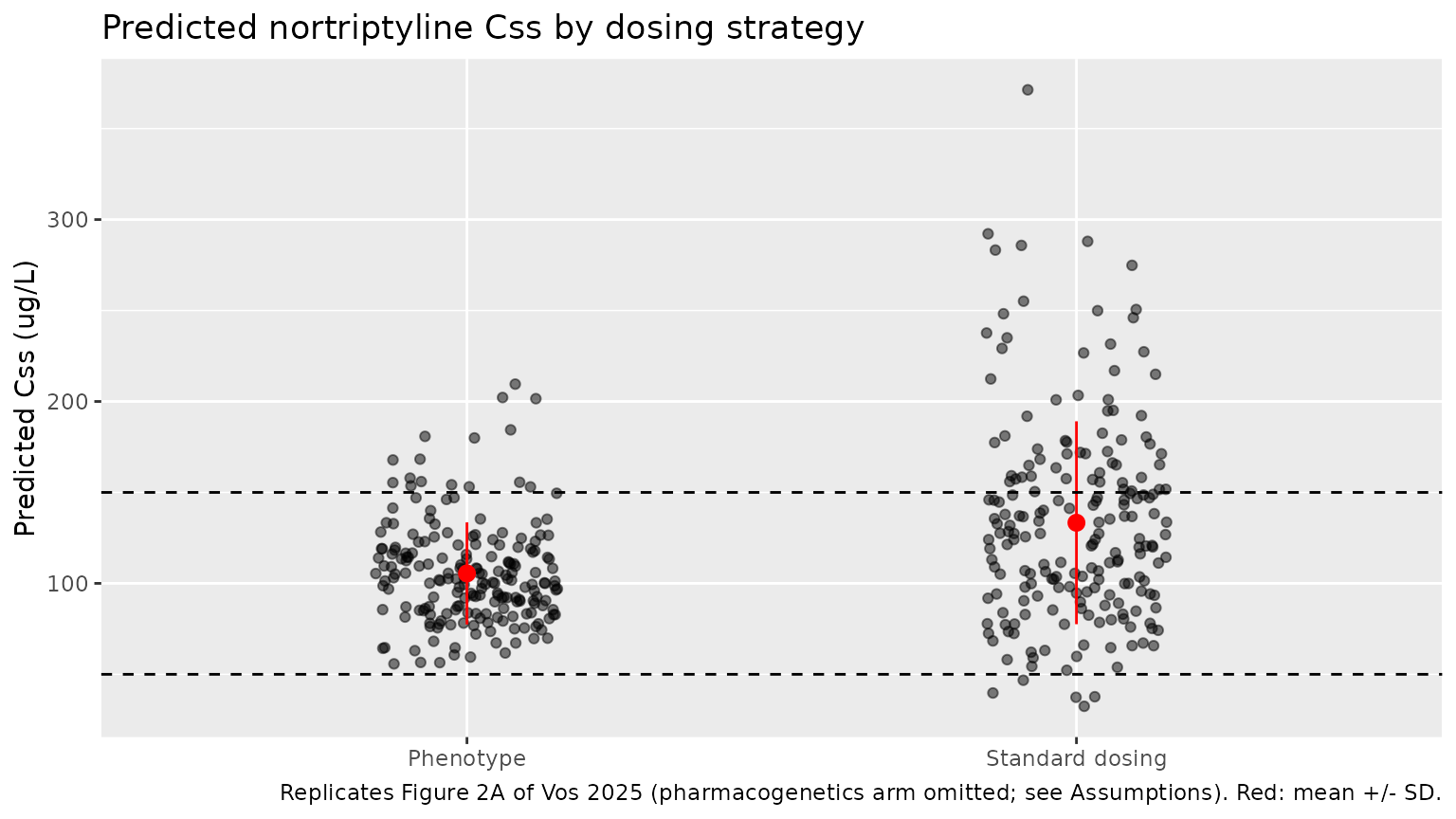
The standard-dosing column reproduces Table 2: the simulated mean (SD) Css and the therapeutic / sub- / supratherapeutic split agree with the published values to within the sampling error of 48 patients. The phenotype-based column reproduces the mean recommended dose and the mean predicted Css. Its spread is narrower than published, so the simulation puts more patients inside the window and fewer above it (about 8% supratherapeutic, against 17%). The virtual patients’ first-dose and one-week concentrations differ only by the model’s 15.6% residual error. Real patients also vary for reasons the model does not carry: adherence, timing errors, a one-week sample that is not quite at steady state, and drift between the two occasions. All of these widen the published distribution. The paper’s own SD ratio between the strategies (59.3 / 37.6 = 1.6) is accordingly smaller than the simulated one.
# Replicates Figure 2A of Vos 2025: predicted Css per dosing strategy.
per_subject |>
  dplyr::select(id, Phenotype = css_pheno, `Standard dosing` = css_standard) |>
  tidyr::pivot_longer(-id, names_to = "strategy", values_to = "css") |>
  ggplot(aes(strategy, css)) +
  geom_jitter(width = 0.15, alpha = 0.5) +
  stat_summary(
    fun = mean, fun.min = function(x) mean(x) - sd(x), fun.max = function(x) mean(x) + sd(x),
    colour = "red"
  ) +
  geom_hline(yintercept = c(50, 150), linetype = "dashed") +
  labs(
    x = NULL, y = "Predicted Css (ug/L)",
    title = "Predicted nortriptyline Css by dosing strategy",
    caption = "Replicates Figure 2A of Vos 2025 (pharmacogenetics arm omitted; see Assumptions). Red: mean +/- SD."
  )
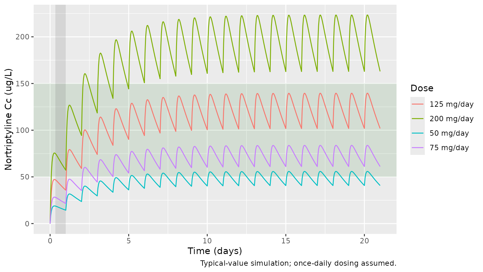
Concentration-time profiles
# Daily-dose profiles for the four doses the genotype-guided strategy assigns
# (50 / 75 / 125 / 200 mg/day for PM / IM / NM / UM), for the typical patient,
# with the 50-150 ug/L therapeutic window and the 8-24 h first-dose sampling
# window shaded.
ev_prof <- dplyr::bind_rows(lapply(c(50, 75, 125, 200), function(d) {
  rxode2::et(amt = d, ii = 24, addl = 20, cmt = "depot") |>
    rxode2::et(seq(0, 504, by = 1), cmt = "central") |>
    as.data.frame() |>
    dplyr::mutate(id = d, dose = paste(d, "mg/day"))
}))
sim_prof <- rxode2::rxSolve(rxode2::zeroRe(mod), ev_prof, keep = "dose") |> as.data.frame()
#> ℹ parameter labels from comments will be replaced by 'label()'
#> ℹ omega/sigma items treated as zero: 'etalclint'
#> Warning: multi-subject simulation without without 'omega'

ggplot(sim_prof, aes(time / 24, Cc, colour = dose)) +
  annotate("rect", xmin = -Inf, xmax = Inf, ymin = 50, ymax = 150, alpha = 0.1, fill = "darkgreen") +
  annotate("rect", xmin = 8 / 24, xmax = 1, ymin = -Inf, ymax = Inf, alpha = 0.15) +
  geom_line() +
  labs(
    x = "Time (days)", y = "Nortriptyline Cc (ug/L)", colour = "Dose",
    caption = "Typical-value simulation; once-daily dosing assumed."
  )
PKNCA validation
The paper reports no NCA. The comparison below uses a 200-patient single 125 mg dose. Because Cmax, tmax, AUC and half-life are all monotone in the one random effect (CLint), their cohort medians should match the typical-value closed forms.
rxode2::rxSetSeed(20250526)
obs_grid <- c(0, 0.5, 1, 2, 3, 4, 5, 6, 8, 10, 12, 16, 24, 36, 48, 72, 96, 120, 168, 240, 336)
ev_sd <- rxode2::et(amt = 125, cmt = "depot") |>
  rxode2::et(obs_grid, cmt = "central") |>
  rxode2::et(id = seq_len(200)) |>
  as.data.frame() |>
  dplyr::mutate(treatment = "125 mg single dose")
sim_sd <- rxode2::rxSolve(mod, ev_sd, keep = "treatment") |> as.data.frame()

sim_nca <- sim_sd |>
  dplyr::filter(!is.na(Cc)) |>
  dplyr::select(id, time, Cc, treatment)
sim_nca <- dplyr::bind_rows(
  sim_nca,
  sim_nca |> dplyr::distinct(id, treatment) |> dplyr::mutate(time = 0, Cc = 0)
) |>
  dplyr::distinct(id, treatment, time, .keep_all = TRUE) |>
  dplyr::arrange(id, treatment, time)

conc_obj <- PKNCA::PKNCAconc(sim_nca, Cc ~ time | treatment + id)
dose_df <- ev_sd |>
  dplyr::filter(evid == 1) |>
  dplyr::select(id, time, amt, treatment)
dose_obj <- PKNCA::PKNCAdose(dose_df, amt ~ time | treatment + id)
intervals <- data.frame(
  start = 0, end = Inf,
  cmax = TRUE, tmax = TRUE, aucinf.obs = TRUE, half.life = TRUE
)
nca_res <- PKNCA::pk.nca(PKNCA::PKNCAdata(conc_obj, dose_obj, intervals = intervals))
ka_tv <- exp(theta[["lka"]])
kel_tv <- cl_tv / vc_tv
tmax_tv <- log(ka_tv / kel_tv) / (ka_tv - kel_tv)
cmax_tv <- conc_single_dose(0, tmax_tv, 125, theta)

reference <- tibble::tibble(
  treatment = "125 mg single dose",
  cmax = cmax_tv,
  tmax = tmax_tv,
  aucinf.obs = 1000 * 125 / clint_tv,
  half.life = thalf_tv
)
cmp <- nlmixr2lib::ncaComparisonTable(
  simulated = nca_res,
  reference = reference,
  by = "treatment",
  units = c(cmax = "ug/L", tmax = "h", aucinf.obs = "h*ug/L", half.life = "h"),
  tolerance_pct = 20
)
knitr::kable(
  cmp,
  caption = "Simulated (median of 200) vs. typical-value closed form. * differs by >20%."
)| NCA parameter | treatment | Reference | Simulated | % diff |
|---|---|---|---|---|
| Cmax (ug/L) | 125 mg single dose | 47.3 | 48.6 | +2.8% |
| Tmax (h) | 125 mg single dose | 6.58 | 6 | -8.8% |
| AUC0-∞ (obs) (h*ug/L) | 125 mg single dose | 2960 | 3110 | +5.2% |
| t½ (h) | 125 mg single dose | 38.5 | 39.5 | +2.5% |
Simulated medians land on the closed-form typical values. The sparse 4-6 h grid around the peak shifts the observed tmax by at most an hour.
Assumptions and deviations
- Dosing frequency. The article gives doses in mg/day without a frequency. All simulations use once-daily dosing; the steady-state sample is placed 12 h after the dose, the midpoint of the protocol’s 10-16 h window.
- First dose for phenotyping. The size of the single phenotyping dose is not reported. With linear PK and a proportional residual error the empirical Bayes estimate does not depend on the dose, so the vignette uses the 125 mg/day regimen throughout.
-
IIV scale. ESM 1 Table A reports the CLint
variability as ‘43.5%’ without saying whether this is the log-normal CV
or
100 * sqrt(omega^2). The model uses the log-normal CV,omega^2 = log(1 + 0.435^2) = 0.173; thesqrt(omega^2)reading would give 0.189, which changes the predicted Css spread by about 4%. - “Css” at one week. The paper treats the one-week concentration as steady state. At the typical half-life the patient is about 94% of the way there, and the vignette’s standard-dosing column samples at one week to match what the paper actually measured.
- Pharmacogenetics-based dosing not replicated. The PK model has no CYP2D6 covariate: genotype entered only through the guideline doses applied to the observed concentrations. A model-based simulation of that arm would need a genotype-to-CLint relation that the paper does not estimate.
- Phenotype-based dose. The paper does not say whether recommended doses were rounded to available tablet strengths; the vignette uses the unrounded dose. The virtual cohort is drawn from the model’s own CLint distribution, whereas the paper’s 48 patients are a subset of the 85 used to fit it.
- Phenotype-arm spread. The simulated phenotype-based Css distribution is narrower than Table 2 reports (see the comparison above), so its therapeutic and supratherapeutic proportions are shown but not used as a validation gate.
- No erratum or correction notice was found in Europe PMC (checked 2026-11-04).