Ivosidenib (Jiang 2021)
Source:vignettes/articles/Jiang_2021_ivosidenib.Rmd
Jiang_2021_ivosidenib.RmdModel and source
- Citation: Jiang X, Wada R, Poland B, Kleijn HJ, Fan B, Liu G, Liu H, Kapsalis S, Yang H, Le K. Population pharmacokinetic and exposure-response analyses of ivosidenib in patients with IDH1-mutant advanced hematologic malignancies. Clin Transl Sci. 2021;14(3):942-953. doi:10.1111/cts.12959
- Description (PK): Two-compartment population PK model for oral ivosidenib (AG-120) in adults with IDH1-mutant advanced hematologic malignancies (mostly relapsed or refractory AML) from the phase 1 AG120-C-001 study (Jiang 2021). Sequential zero-order release into the depot followed by first-order absorption; first-order elimination. The model is parameterised on steady-state apparent parameters at 500 mg once daily, with a step change between the first dose and repeated dosing (a 0.50-fold change in relative bioavailability and a 1.66-fold change in clearance, MULTI_DOSE_PT), a less-than-dose- proportional power effect of dose on relative bioavailability, baseline-albumin and albumin-ratio power effects on CL/F and Vc/F, a baseline body-weight power effect on Vc/F, and multiplicative CYP3A4-inhibitor effects on CL/F (voriconazole, fluconazole, posaconazole, other moderate/strong and mild inhibitors). The concentration-QTcF model of the same paper is packaged separately as Jiang_2021_ivosidenib_QTcF.
- Description (C-QTc): Linear concentration-QTc model relating the change from baseline in the Fridericia-corrected QT interval (DeltaQTcF, ms) to the plasma ivosidenib concentration, pooled across the phase 1 studies AG120-C-001 (IDH1-mutant hematologic malignancies), AG120-C-002 (IDH1-mutant solid tumors) and AG120-C-004 (healthy volunteers) (Jiang 2021). Direct effect with no hysteresis: DeltaQTcF = e0 + slope * CP_IVOSIDENIB_NGML. Typical-value model only: the paper reports the slope (0.00258 ms per ng/mL) and the predicted DeltaQTcF at the 500 mg once-daily geometric-mean Cmax (17.2 ms at 6551 ng/mL), from which the intercept is back-solved; the between-subject variances of the intercept and slope, the residual error, and the intercept covariate coefficients are not reported. PD-only model: the ivosidenib concentration is supplied as a time-varying covariate, for example from a simulation of Jiang_2021_ivosidenib.
- Article (open access): https://doi.org/10.1111/cts.12959
Jiang 2021 reports three analyses of the phase 1 ivosidenib programme:
- a population PK model (packaged as
Jiang_2021_ivosidenib); - exposure-efficacy and exposure-safety analyses based on the post hoc steady-state AUC, which found no exposure-response relationship and so produced no final exposure-response model to package; and
- a linear concentration-QTcF model fitted to a pooled dataset of
three phase 1 studies (packaged as
Jiang_2021_ivosidenib_QTcF).
Population
The population PK analysis used 4656 plasma concentrations from 253 adults with IDH1-mutant advanced hematologic malignancies enrolled in the phase 1 study AG120-C-001 (NCT02074839). In the dose-escalation phase patients received 100 mg twice daily or 300, 500, 800 or 1200 mg once daily in continuous 28-day cycles, and the first three patients of each cohort also received a single dose on day -3; in the expansion phase all patients received 500 mg once daily (225 of 255 patients at the approved 500 mg dose). Supplementary Table S1 (N = 255) reports 54% men, 69% White (20% race missing), median age 68 years (18-89), median weight 74.2 kg (37.7-150.4), median baseline albumin 37 g/L (15-48) and median creatinine clearance 83 mL/min/1.73 m^2. Most patients had relapsed or refractory AML (80%) and an ECOG performance status of 0 or 1 (78%). Supplementary Table S2 counts the concentration samples taken with concomitant voriconazole (21%), fluconazole (18%), posaconazole (6%), other moderate/strong CYP3A4 inhibitors (6%) and mild CYP3A4 inhibitors (24%).
The concentration-QTcF analysis pooled 1203 triplicate ECGs with time-matched plasma concentrations from 171 participants in AG120-C-001, AG120-C-002 (IDH1-mutant advanced solid tumors) and AG120-C-004 (healthy volunteers).
The same information is available programmatically via
readModelDb("Jiang_2021_ivosidenib")()$population.
Source trace
Every ini() value carries an in-file comment pointing to
its source. The table collects them.
| Equation / parameter | Value | Source location |
|---|---|---|
| Structure: 2-compartment, zero-order release into depot then first-order absorption | n/a | Results ‘Base population PK model’; Figure 1a |
lcl (steady-state CL/F) |
log(5.39 L/h) | Table 1 |
lvc (steady-state Vc/F) |
log(234 L) | Table 1 |
lq (steady-state Q/F) |
log(15.8 L/h) | Table 1 |
lvp (steady-state Vp/F) |
log(151 L) | Table 1 |
lka |
log(1.38 1/h) | Table 1 |
ld1 (zero-order release duration) |
log(0.27 h) | Table 1 ‘Tlag’, footnote ‘zero-order release duration (lag-time)’ |
e_multi_dose_pt_f |
0.50 | Table 1 ‘Steady-state fold change in Frel’ |
e_md_cl |
1.66 | Table 1 ‘Steady-state fold change in CL’ |
e_dose_fdepot |
-0.49 | Table 1 ‘Dose-Frel exponent’; reference 500 mg from Figure 2 |
e_wt_vc |
0.92 | Table 1; reference 74.2 kg from Figure 2b |
e_alb_base_cl, e_alb_ratio_cl
|
0.82, 0.99 | Table 1; reference 37 g/L from Figure 2 |
e_alb_base_vc, e_alb_ratio_vc
|
0.73, 1.1 | Table 1 |
e_conmed_voriconazole_cl |
0.64 | Table 1 |
e_conmed_fluconazole_cl |
0.59 | Table 1 |
e_conmed_posaconazole_cl |
0.65 | Table 1 |
e_conmed_cyp3a4_inh_modstrong_cl |
0.92 | Table 1 ‘other moderate/strong CYP3A inhibitors’ |
e_conmed_cyp3a4_inh_weak_cl |
1.04 | Table 1 ‘mild CYP3A inhibitors’ |
etalcl, etalvc, etalka
|
0.35^2, 0.47^2, 1.08^2 | Table 1 BSV CV% 35, 47, 108 |
expSd |
0.26 | Table 1 ‘Log-additive CV%’ = 26 |
First-dose step cl * 1.66^(MULTI_DOSE_PT - 1),
F * 0.50^(MULTI_DOSE_PT - 1)
|
n/a | Results ‘Final population PK model’; Figure 1a; Figure S1c |
slope (C-QTc) |
0.00258 ms per ng/mL | Results ‘QTc analysis’ |
e0 (C-QTc) |
0.30 ms | Back-solved: 17.2 - 0.00258 * 6551 (Results ‘QTc analysis’) |
How the first-dose step is encoded
The authors parameterised the model on steady-state apparent
parameters and described the change from the first dose to repeated
dosing as “a 2-fold decrease in relative bioavailability and a 1.66-fold
increase in CL/F, such that the net change in apparent CL was 3.3-fold”
(Results). Figure 1a places a day-1 and a steady-state value on exactly
two quantities, Frel and CL, and Supplementary
Figure S1c states that the two factors begin to act at the start of
continuous once-daily dosing. In the packaged model,
MULTI_DOSE_PT = 0 from the first dose until the second
dose, and 1 afterwards; at 0 the dose’s bioavailability is 2-fold and
clearance is 1/1.66-fold the steady-state values. This reproduces the
printed first-dose CL/F:
first_dose_clf <- 5.39 / ((1 / 0.50) * 1.66)
first_dose_clf
#> [1] 1.623494
stopifnot(abs(first_dose_clf - 1.63) < 0.01)
Table 1 also prints derived first-dose values for Vc/F (71 L), Q/F
(4.8 L/h) and Vp/F (46 L). Each is the steady-state value divided by the
full 3.3-fold factor, which would mean the clearance factor also scales
both volumes and the intercompartmental clearance. That contradicts the
text and Figure 1a, where only Frel and CL
change. Under the model as described, the first-dose apparent volumes
are the steady-state values divided by the 2-fold bioavailability change
alone (Vc/F = 117 L, Q/F = 7.9 L/h, Vp/F = 75.5 L).
The two readings can be told apart using quantities the paper prints independently: the single-dose half-life “of 72-138 h” and the median single-dose Tmax range of 2.4-5.5 h (Introduction, from the phase 1 NCA). The chunk below simulates a typical 500 mg single dose under both readings.
mod <- readModelDb("Jiang_2021_ivosidenib")
mod_typ <- rxode2::zeroRe(mod)
#> ℹ parameter labels from comments will be replaced by 'label()'

# The Table-1-derived reading: every disposition parameter divided by 3.3.
# Written out explicitly because it is not the packaged structure.
table_reading <- rxode2::rxode2({
  d/dt(depot) <- -ka * depot
  d/dt(central) <- ka * depot - cl / vc * central - q / vc * central + q / vp * peripheral1
  d/dt(peripheral1) <- q / vc * central - q / vp * peripheral1
  dur(depot) <- d1
  Cc <- central / vc * 1000
})

single_dose_events <- function(extra = list()) {
  obs_t <- sort(unique(c(seq(0, 12, by = 0.05), seq(12.5, 72, by = 0.5))))
  ev <- dplyr::bind_rows(
    data.frame(id = 1L, time = 0, evid = 1L, amt = 500, rate = -2, cmt = "depot"),
    data.frame(id = 1L, time = obs_t, evid = 0L, amt = 0, rate = 0, cmt = "central")
  )
  ev <- dplyr::mutate(ev, DOSE = 500, MULTI_DOSE_PT = 0L, WT = 74.2,
                      ALB_BASE = 37, ALB = 37,
                      CONMED_VORICONAZOLE = 0L, CONMED_FLUCONAZOLE = 0L,
                      CONMED_POSACONAZOLE = 0L, CONMED_CYP3A4_INH_MOD = 0L,
                      CONMED_CYP3A4_INH_STRONG = 0L, CONMED_CYP3A4_INH_WEAK = 0L)
  dplyr::arrange(ev, time, dplyr::desc(evid))
}

summarise_single_dose <- function(s, label) {
  s <- as.data.frame(s)
  c48 <- s$Cc[abs(s$time - 48) < 1e-6]
  c72 <- s$Cc[abs(s$time - 72) < 1e-6]
  data.frame(
    reading = label,
    cmax = max(s$Cc),
    tmax = s$time[which.max(s$Cc)],
    c72 = c72,
    thalf_48_72 = 24 * log(2) / log(c48 / c72)
  )
}

sd_model <- rxode2::rxSolve(mod_typ, single_dose_events(), returnType = "data.frame")
#> ℹ omega/sigma items treated as zero: 'etalcl', 'etalvc', 'etalka'
sd_table <- rxode2::rxSolve(
  table_reading,
  params = c(ka = 1.38, d1 = 0.27, cl = 1.63, vc = 71, q = 4.8, vp = 46),
  events = single_dose_events(), returnType = "data.frame"
)

readings <- dplyr::bind_rows(
  summarise_single_dose(sd_model, "Packaged model (only F and CL change)"),
  summarise_single_dose(sd_table, "Table 1 derived first-dose rows (all divided by 3.3)")
)

readings |>
  dplyr::mutate(dplyr::across(c(cmax, c72), \(x) round(x))) |>
  dplyr::mutate(dplyr::across(c(tmax, thalf_48_72), \(x) round(x, 1))) |>
  dplyr::rename("Reading" = reading, "Cmax (ng/mL)" = cmax, "Tmax (h)" = tmax,
                "C72h (ng/mL)" = c72, "Half-life 48-72 h (h)" = thalf_48_72) |>
knitr::kable(caption = "Typical 500 mg single dose under the two readings.")| Reading | Cmax (ng/mL) | Tmax (h) | C72h (ng/mL) | Half-life 48-72 h (h) |
|---|---|---|---|---|
| Packaged model (only F and CL change) | 3613 | 2.4 | 1359 | 84.8 |
| Table 1 derived first-dose rows (all divided by 3.3) | 5867 | 2.4 | 1491 | 52.5 |
stopifnot(
  # The packaged reading lands inside the printed single-dose half-life range.
  readings$thalf_48_72[1] > 72, readings$thalf_48_72[1] < 138,
  # The Table-1-derived reading does not.
  readings$thalf_48_72[2] < 72,
  # Tmax sits within the printed 2.4-5.5 h single-dose range (packaged model).
  readings$tmax[1] >= 2.3, readings$tmax[1] <= 5.5
)
The packaged reading gives a 48-72 h half-life of about 85 h and a single-dose Cmax of about 3600 ng/mL, consistent with the observed day -3 mean profile of Supplementary Figure S1b (peak near 3000 ng/mL) and the median line of the first-dose panel of Figure 1b (near 3300 ng/mL). The Table-1-derived reading gives a 52 h half-life, outside the printed range, and a Cmax near 5900 ng/mL. The first-dose volume rows of Table 1 are therefore treated as a derivation slip in the table; they are not model inputs in either case, because the model is parameterised on the steady-state values.
Typical-value replication of Figure 2
Figure 2 gives the steady-state AUC for the typical patient (500 mg once daily, albumin 37 g/L, no CYP3A4 inhibitor; 93 ug*h/mL) and for one-at-a-time covariate changes (Figure 2c table), and the typical steady-state Cmax (4827 ng/mL, weight 74.2 kg). The chunk below simulates each scenario to steady state with the random effects removed and computes AUC0-24 and Cmax with PKNCA over the day-20 dosing interval.
ref_cov <- data.frame(
  DOSE = 500, WT = 74.2, ALB_BASE = 37, ALB = 37,
  CONMED_VORICONAZOLE = 0L, CONMED_FLUCONAZOLE = 0L, CONMED_POSACONAZOLE = 0L,
  CONMED_CYP3A4_INH_MOD = 0L, CONMED_CYP3A4_INH_STRONG = 0L,
  CONMED_CYP3A4_INH_WEAK = 0L
)

# Published Figure 2c AUC estimates (ug*h/mL) for each one-at-a-time change.
scenarios <- tibble::tribble(
  ~scenario,                ~var,                   ~value, ~auc_pub,
  "Typical patient",        "DOSE",                 500,    93,
  "Dose 300 mg",            "DOSE",                 300,    71,
  "Dose 800 mg",            "DOSE",                 800,    118,
  "Voriconazole",           "CONMED_VORICONAZOLE",  1,      145,
  "Fluconazole",            "CONMED_FLUCONAZOLE",   1,      157,
  "Posaconazole",           "CONMED_POSACONAZOLE",  1,      142,
  "Albumin baseline 26 g/L", "ALB_BASE",            26,     124,
  "Albumin baseline 44 g/L", "ALB_BASE",            44,     80,
  "Albumin ratio 0.84",     "ALB",                  0.84 * 37, 111,
  "Albumin ratio 1.24",     "ALB",                  1.24 * 37, 75
) |>
  dplyr::mutate(id = dplyr::row_number())

# Scenario covariates: the reference patient with one column changed. For the
# baseline-albumin scenarios the time-varying albumin moves with it (ratio 1).
scen_cov <- dplyr::bind_rows(lapply(seq_len(nrow(scenarios)), \(i) {
  cv <- ref_cov
  cv[[scenarios$var[i]]] <- scenarios$value[i]
  if (scenarios$var[i] == "ALB_BASE") cv$ALB <- scenarios$value[i]
  cv$id <- scenarios$id[i]
  cv
}))

build_events <- function(cov, dose_times, obs_times) {
  second_dose <- dose_times[2]
  doses <- tidyr::crossing(id = cov$id, time = dose_times) |>
    dplyr::mutate(evid = 1L, rate = -2, cmt = "depot")
  obs <- tidyr::crossing(id = cov$id, time = obs_times) |>
    dplyr::mutate(evid = 0L, rate = 0, cmt = "central")
  dplyr::bind_rows(doses, obs) |>
    dplyr::left_join(cov, by = "id") |>
    dplyr::mutate(
      amt = dplyr::if_else(evid == 1L, DOSE, 0),
      MULTI_DOSE_PT = as.integer(time >= second_dose)
    ) |>
    dplyr::select(id, time, evid, amt, rate, cmt, dplyr::everything()) |>
    dplyr::arrange(id, time, dplyr::desc(evid))
}

qd_times <- seq(0, 19 * 24, by = 24)
ss_start <- 19 * 24
ss_obs <- ss_start + sort(unique(c(seq(0, 6, by = 0.05), seq(6.5, 24, by = 0.5))))
ev_scen <- build_events(scen_cov, qd_times, ss_obs)
sim_scen <- rxode2::rxSolve(mod_typ, events = ev_scen, returnType = "data.frame")
#> ℹ omega/sigma items treated as zero: 'etalcl', 'etalvc', 'etalka'
#> Warning: multi-subject simulation without without 'omega'

conc_scen <- PKNCA::PKNCAconc(
  dplyr::select(sim_scen, id, time, Cc), Cc ~ time | id
)
dose_scen <- PKNCA::PKNCAdose(
  dplyr::filter(ev_scen, evid == 1L) |> dplyr::select(id, time, amt),
  amt ~ time | id
)
int_scen <- data.frame(start = ss_start, end = ss_start + 24,
                       cmax = TRUE, auclast = TRUE)
nca_scen <- PKNCA::pk.nca(PKNCA::PKNCAdata(conc_scen, dose_scen, intervals = int_scen))

fig2 <- as.data.frame(nca_scen$result) |>
  dplyr::select(id, PPTESTCD, PPORRES) |>
  tidyr::pivot_wider(names_from = PPTESTCD, values_from = PPORRES) |>
  dplyr::inner_join(scenarios, by = "id") |>
  dplyr::mutate(auc_model = auclast / 1000,
                pct_diff = 100 * (auc_model - auc_pub) / auc_pub)
stopifnot(nrow(fig2) == nrow(scenarios))

fig2 |>
  dplyr::transmute(scenario, auc_pub, auc_model = round(auc_model, 1),
                   pct_diff = round(pct_diff, 1), cmax = round(cmax)) |>
  dplyr::rename("Scenario" = scenario, "Published AUCss (ug*h/mL)" = auc_pub,
                "Model AUCss (ug*h/mL)" = auc_model, "% difference" = pct_diff,
                "Model Cmax,ss (ng/mL)" = cmax) |>
knitr::kable(caption = "Replicates the Figure 2c table of Jiang 2021 (typical values).")| Scenario | Published AUCss (ug*h/mL) | Model AUCss (ug*h/mL) | % difference | Model Cmax,ss (ng/mL) |
|---|---|---|---|---|
| Typical patient | 93 | 92.7 | -0.3 | 4823 |
| Dose 300 mg | 71 | 71.4 | 0.6 | 3717 |
| Dose 800 mg | 118 | 117.8 | -0.2 | 6130 |
| Voriconazole | 145 | 143.3 | -1.1 | 6916 |
| Fluconazole | 157 | 154.8 | -1.4 | 7387 |
| Posaconazole | 142 | 141.2 | -0.5 | 6829 |
| Albumin baseline 26 g/L | 124 | 123.6 | -0.3 | 6406 |
| Albumin baseline 44 g/L | 80 | 80.4 | 0.5 | 4195 |
| Albumin ratio 0.84 | 111 | 110.1 | -0.8 | 5762 |
| Albumin ratio 1.24 | 75 | 74.9 | -0.1 | 3873 |
typ_cmax <- fig2$cmax[fig2$scenario == "Typical patient"]
stopifnot(
  # Typical-value solves use the same parameters the paper's table was
  # generated from; the only differences are the paper's rounding of the
  # printed estimates and of the AUCs (realised max |diff| about 1%).
  max(abs(fig2$pct_diff)) < 3,
  abs(typ_cmax - 4827) / 4827 < 0.02
)
Every row matches the published AUC within rounding, which confirms the reference dose (500 mg), the reference albumin (37 g/L), the positive sign of the albumin exponents, the ratio form of the within-subject albumin effect and the multiplicative CYP3A4-inhibitor fold changes. The typical Cmax matches the 4827 ng/mL of Figure 2b, which also exercises the Vc/F covariates.
Virtual cohorts
Two cohorts of 200 participants each, all at 500 mg:
- Reference cohort – covariates at the Figure 2 reference values, with between-subject variability. This approximates the prediction-corrected VPC of Figure 1b. The design follows the dose-escalation schedule: a single dose at time 0 (day -3), then continuous once-daily dosing from 72 h (cycle 1 day 1).
- Covariate cohort – baseline weight, baseline albumin, albumin ratio and CYP3A4-inhibitor use drawn to approximate Supplementary Tables S1 and S2, used for the population AUC and Cmax ranges of Figure 2.
set.seed(20210301)
rxode2::rxSetSeed(20210301)
n <- 200

ref_cohort <- ref_cov[rep(1, n), ] |>
  dplyr::mutate(id = seq_len(n))

# Covariate cohort. Weight: log-normal, median 74.2 kg, CV 24%, truncated to
# the observed range. Baseline albumin: normal, mean 36 g/L, CV 16%, truncated
# to 15-48 g/L. Albumin ratio: log-normal matching the Figure 2 5th-95th
# percentiles of 0.84-1.24. CYP3A4 inhibitors: one of voriconazole /
# fluconazole / posaconazole / other moderate-strong / none with the Table S2
# sample fractions, plus an independent mild-inhibitor draw.
rtrunc <- function(x, lo, hi) pmin(pmax(x, lo), hi)
inh <- sample(c("vori", "fluc", "posa", "other", "none"), n, replace = TRUE,
              prob = c(0.21, 0.18, 0.06, 0.06, 0.49))
alb_base <- rtrunc(rnorm(n, 36, 0.16 * 36), 15, 48)
alb_ratio <- exp(rnorm(n, log(sqrt(0.84 * 1.24)), log(1.24 / 0.84) / (2 * 1.645)))
cov_cohort <- data.frame(
  id = n + seq_len(n),
  DOSE = 500,
  WT = rtrunc(exp(rnorm(n, log(74.2), 0.237)), 37.7, 150.4),
  ALB_BASE = alb_base,
  ALB = alb_base * alb_ratio,
  CONMED_VORICONAZOLE = as.integer(inh == "vori"),
  CONMED_FLUCONAZOLE = as.integer(inh == "fluc"),
  CONMED_POSACONAZOLE = as.integer(inh == "posa"),
  CONMED_CYP3A4_INH_MOD = as.integer(inh == "other"),
  CONMED_CYP3A4_INH_STRONG = 0L,
  CONMED_CYP3A4_INH_WEAK = rbinom(n, 1, 0.24)
)

# Reference cohort: day -3 single dose at t = 0, once daily from 72 h (C1D1)
# through C1D28. First-dose panel 0-72 h; C1D15 steady-state panel 408-432 h.
dose_times_esc <- c(0, seq(72, 72 + 27 * 24, by = 24))
c1d15 <- 72 + 14 * 24
obs_esc <- sort(unique(c(
  seq(0, 12, by = 0.25), seq(13, 72, by = 1),
  c1d15 + c(seq(0, 12, by = 0.25), seq(13, 24, by = 1))
)))
ev_ref <- build_events(ref_cohort, dose_times_esc, obs_esc)

# Covariate cohort: once daily from time 0; only the day-15 interval observed.
ss15 <- 14 * 24
ev_cov <- build_events(cov_cohort, seq(0, 20 * 24, by = 24),
                       ss15 + c(seq(0, 12, by = 0.25), seq(13, 24, by = 1)))

stopifnot(
  !anyDuplicated(unique(ev_ref[, c("id", "time", "evid")])),
  !anyDuplicated(unique(ev_cov[, c("id", "time", "evid")])),
  length(intersect(ev_ref$id, ev_cov$id)) == 0
)Replicate Figure 1b (visual predictive check)
vpc <- sim_ref |>
  dplyr::mutate(panel = dplyr::case_when(
    time <= 72 ~ "First dose (day -3)",
    time >= c1d15 & time <= c1d15 + 24 ~ "Steady state (C1D15)",
    TRUE ~ NA_character_
  )) |>
  dplyr::filter(!is.na(panel)) |>
  dplyr::mutate(tad = dplyr::if_else(panel == "First dose (day -3)", time, time - c1d15)) |>
  dplyr::group_by(panel, tad) |>
  dplyr::summarise(Q05 = quantile(Cc, 0.05), Q50 = quantile(Cc, 0.50),
                   Q95 = quantile(Cc, 0.95), .groups = "drop")

ggplot(vpc, aes(tad, Q50)) +
  geom_ribbon(aes(ymin = Q05, ymax = Q95), alpha = 0.25, fill = "steelblue") +
  geom_line(colour = "firebrick") +
  facet_wrap(~panel, scales = "free_x") +
  scale_y_log10(limits = c(200, 10000)) +
  labs(x = "Time after dose (h)", y = "Ivosidenib concentration (ng/mL)",
       title = "Simulated 5th, 50th and 95th percentiles, 500 mg",
       caption = "Replicates Figure 1b of Jiang 2021 (reference covariates; 200 participants).")
#> Warning in scale_y_log10(limits = c(200, 10000)): log-10 transformation introduced infinite values.
#> log-10 transformation introduced infinite values.
#> log-10 transformation introduced infinite values.
#> log-10 transformation introduced infinite values.
#> Warning: Removed 1 row containing missing values or values outside the scale range
#> (`geom_ribbon()`).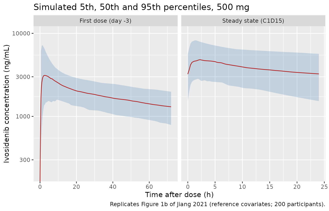
After the first dose the simulated median peaks near 3100 ng/mL and falls to about 1300 ng/mL at 72 h, with a 90% interval of roughly 1400-7500 ng/mL at the peak; the first-dose panel of Figure 1b shows a median near 3300 ng/mL at the peak and 1600 ng/mL at 72 h, with a 95th percentile near 7000 ng/mL. The steady-state panel here is the C1D15 dosing interval only, with a median peak near 4800 ng/mL. The right panel of Figure 1b is not a like-for-like comparator: it pools every sample after the first dose (including pre-steady-state days and pre-dose samples plotted at about 24 h) and is prediction-corrected across dose levels, so its median (about 3300 ng/mL at the peak) sits below a pure steady-state profile.
PKNCA validation
nca_conc <- sim_ref |>
  dplyr::filter(!is.na(Cc)) |>
  dplyr::mutate(arm = "500 mg") |>
  dplyr::select(id, time, Cc, arm)
# The event table observes at t = 0 for every participant, so the time-zero
# anchor PKNCA needs is already present.
stopifnot(all(tapply(nca_conc$time, nca_conc$id, min) == 0))

nca_dose <- ev_ref |>
  dplyr::filter(evid == 1L) |>
  dplyr::mutate(arm = "500 mg") |>
  dplyr::select(id, time, amt, arm)

conc_obj <- PKNCA::PKNCAconc(nca_conc, Cc ~ time | arm + id, concu = "ng/mL", timeu = "h")
dose_obj <- PKNCA::PKNCAdose(nca_dose, amt ~ time | arm + id, doseu = "mg")

# Row 1: the day -3 single dose (0-72 h, before continuous dosing starts).
# Row 2: the C1D15 dosing interval.
intervals <- data.frame(
  start     = c(0,     c1d15),
  end       = c(72,    c1d15 + 24),
  cmax      = c(TRUE,  TRUE),
  tmax      = c(TRUE,  TRUE),
  auclast   = c(FALSE, TRUE),
  cmin      = c(FALSE, TRUE),
  half.life = c(TRUE,  FALSE)
)
nca_res <- PKNCA::pk.nca(PKNCA::PKNCAdata(conc_obj, dose_obj, intervals = intervals))

nca_tab <- as.data.frame(nca_res$result) |>
  dplyr::mutate(period = dplyr::if_else(start == 0, "First dose", "Steady state"))

nca_tab |>
  dplyr::group_by(period, PPTESTCD) |>
  dplyr::summarise(median = stats::median(PPORRES, na.rm = TRUE),
                   p05 = stats::quantile(PPORRES, 0.05, na.rm = TRUE),
                   p95 = stats::quantile(PPORRES, 0.95, na.rm = TRUE),
                   .groups = "drop") |>
  dplyr::mutate(dplyr::across(c(median, p05, p95), \(x) signif(x, 3))) |>
  dplyr::rename("Period" = period, "Parameter" = PPTESTCD, "Median" = median,
                "5th percentile" = p05, "95th percentile" = p95) |>
knitr::kable(caption = "PKNCA summary, reference cohort (500 mg).")| Period | Parameter | Median | 5th percentile | 95th percentile |
|---|---|---|---|---|
| First dose | adj.r.squared | 1.00e+00 | 1.00e+00 | 1.00e+00 |
| First dose | clast.pred | 1.30e+03 | 7.89e+02 | 1.98e+03 |
| First dose | cmax | 3.33e+03 | 1.70e+03 | 7.27e+03 |
| First dose | half.life | 8.67e+01 | 4.70e+01 | 1.79e+02 |
| First dose | lambda.z | 7.99e-03 | 3.88e-03 | 1.47e-02 |
| First dose | lambda.z.n.points | 4.30e+01 | 3.60e+01 | 5.20e+01 |
| First dose | lambda.z.time.first | 3.00e+01 | 2.10e+01 | 3.70e+01 |
| First dose | lambda.z.time.last | 7.20e+01 | 7.20e+01 | 7.20e+01 |
| First dose | r.squared | 1.00e+00 | 1.00e+00 | 1.00e+00 |
| First dose | span.ratio | 4.87e-01 | 1.98e-01 | 1.04e+00 |
| First dose | tlast | 7.20e+01 | 7.20e+01 | 7.20e+01 |
| First dose | tmax | 2.00e+00 | 7.50e-01 | 7.81e+00 |
| Steady state | auclast | 9.26e+04 | 5.25e+04 | 1.52e+05 |
| Steady state | cmax | 4.98e+03 | 2.84e+03 | 8.44e+03 |
| Steady state | cmin | 3.23e+03 | 1.53e+03 | 5.61e+03 |
| Steady state | tmax | 1.75e+00 | 7.50e-01 | 5.52e+00 |
Comparison against published values
Jiang 2021 prints the model-predicted steady-state AUC (93 ug*h/mL) and Cmax (4827 ng/mL) for the typical patient at 500 mg (Figure 2). The reference cohort holds every covariate at those typical values, so its median is the right comparator for them.
ss_res <- nca_res
ss_res$result <- dplyr::filter(as.data.frame(nca_res$result), start == c1d15)

published <- tibble::tribble(
  ~arm,     ~cmax, ~auclast,
  "500 mg", 4827,  93000
)

cmp <- nlmixr2lib::ncaComparisonTable(
  simulated = ss_res,
  reference = published,
  by = "arm",
  params = c("cmax", "auclast"),
  units = c(cmax = "ng/mL", auclast = "ng*h/mL"),
  tolerance_pct = 20
)
knitr::kable(
  cmp,
  caption = paste("Simulated (PKNCA, C1D15 dosing interval) versus the",
                  "typical-patient values of Jiang 2021 Figure 2.",
                  "* differs from reference by >20%."),
  align = c("l", "l", "r", "r", "r")
)| NCA parameter | arm | Reference | Simulated | % diff |
|---|---|---|---|---|
| Cmax (ng/mL) | 500 mg | 4830 | 4980 | +3.2% |
| AUClast (ng*h/mL) | 500 mg | 93000 | 92600 | -0.5% |
med <- nca_tab |>
  dplyr::group_by(period, PPTESTCD) |>
  dplyr::summarise(median = stats::median(PPORRES, na.rm = TRUE), .groups = "drop")
get_med <- function(p, code) {
  v <- med$median[med$period == p & med$PPTESTCD == code]
  if (length(v) != 1L) stop("no unique median for ", p, " / ", code)
  v
}
stopifnot(
  # Centre of the cohort against the typical values (robust to the draw).
  abs(get_med("Steady state", "auclast") / 93000 - 1) < 0.10,
  abs(get_med("Steady state", "cmax") / 4827 - 1) < 0.10,
  # Printed single-dose half-life range 72-138 h and Tmax ranges
  # (single dose 2.4-5.5 h; repeated dosing 1.9-4.0 h), Introduction.
  get_med("First dose", "half.life") > 60, get_med("First dose", "half.life") < 150,
  get_med("First dose", "tmax") > 1.2, get_med("First dose", "tmax") < 5.5,
  get_med("Steady state", "tmax") > 1.2, get_med("Steady state", "tmax") < 4.0
)
The cohort median steady-state AUC0-24 and Cmax agree with the typical-patient values, and the first-dose half-life (PKNCA terminal fit over the 0-72 h window, median about 87 h) sits inside the 72-138 h single-dose range printed in the Introduction. The median Tmax is about 2.0 h after the first dose and 1.75 h at steady state, slightly below the printed ranges of median Tmax by dose cohort (2.4-5.5 h single dose, 1.9-4.0 h repeated dosing). Those ranges come from escalation cohorts of three or more patients sampled at 0.5, 1, 2, 3, 4, 6 and 8 h, which places every observed Tmax on a sampling time; the typical-value Tmax of the packaged model is 2.4 h after a single dose (checked exactly above). The cohort assertion below therefore uses 1.2 h as its lower bound (realised medians 2.0 and 1.75 h on a 0.25 h grid).
Replicate the Figure 2 population ranges
The hatched bars of Figure 2 give the 5th-95th percentiles of the modelled steady-state AUC (56-177 ug*h/mL) and Cmax (3023-9102 ng/mL) across the analysis population. The covariate cohort approximates that population.
cov_nca <- sim_cov |>
  dplyr::filter(time >= ss15, time <= ss15 + 24) |>
  dplyr::group_by(id) |>
  dplyr::arrange(time, .by_group = TRUE) |>
  dplyr::summarise(
    cmax = max(Cc),
    auc = sum(diff(time) * (head(Cc, -1) + tail(Cc, -1)) / 2) / 1000,
    .groups = "drop"
  )

pop_range <- data.frame(
  metric = c("AUCss (ug*h/mL)", "Cmax,ss (ng/mL)"),
  published_p05 = c(56, 3023),
  model_p05 = c(quantile(cov_nca$auc, 0.05), quantile(cov_nca$cmax, 0.05)),
  model_median = c(median(cov_nca$auc), median(cov_nca$cmax)),
  published_p95 = c(177, 9102),
  model_p95 = c(quantile(cov_nca$auc, 0.95), quantile(cov_nca$cmax, 0.95))
)
pop_range |>
  dplyr::mutate(dplyr::across(-metric, \(x) signif(x, 3))) |>
  dplyr::rename("Metric" = metric, "Published 5th" = published_p05,
                "Model 5th" = model_p05, "Model median" = model_median,
                "Published 95th" = published_p95, "Model 95th" = model_p95) |>
knitr::kable(caption = "Population 5th-95th percentiles, covariate cohort versus Figure 2.")| Metric | Published 5th | Model 5th | Model median | Published 95th | Model 95th |
|---|---|---|---|---|---|
| AUCss (ug*h/mL) | 56 | 55.7 | 117 | 177 | 208 |
| Cmax,ss (ng/mL) | 3020 | 3280.0 | 5860 | 9100 | 10200 |
stopifnot(
  # Robust quantiles only; the published range comes from post hoc estimates
  # of the real population, which this cohort approximates. Realised on the
  # authoring machine: 5th percentiles -1% (AUC) and +8% (Cmax), 95th
  # percentiles +17% (AUC) and +12% (Cmax). The upper tail depends on how
  # many participants the cohort puts on a CYP3A4 inhibitor, which Table S2
  # gives per sample rather than per patient, so the bound is 30%. A
  # mis-transcribed CL/F, dose or unit moves both tails by far more.
  abs(pop_range$model_p05 / pop_range$published_p05 - 1) < 0.30,
  abs(pop_range$model_p95 / pop_range$published_p95 - 1) < 0.30
)
The simulated 5th percentiles match Figure 2 closely; the 95th percentiles are 12-17% above it. The cohort draws inhibitor use from the per-sample fractions of Table S2 (about half the cohort is on voriconazole, fluconazole or posaconazole for the whole interval), which likely overstates the per-patient steady-state exposure to those azoles. The AUC here is a trapezoidal sum on the dense simulated grid, used only to read the population percentiles; the PKNCA validation above is the NCA of record.
Concentration-QTcF model
The packaged C-QTc model is
DeltaQTcF = e0 + slope * CP_IVOSIDENIB_NGML. At the 500 mg
geometric-mean Cmax of 6551 ng/mL it returns the published 17.2 ms, by
construction of the back-solved intercept. The chunk below replicates
the regression line of Figure 5 and then drives the model with the
simulated steady-state concentrations of the reference cohort.
mod_qt <- readModelDb("Jiang_2021_ivosidenib_QTcF")

conc_grid <- c(0, 1000, 2500, 5000, 6551, 10000, 15000, 20000, 22500)
ev_qt <- data.frame(id = seq_along(conc_grid), time = 0, evid = 0L,
                    CP_IVOSIDENIB_NGML = conc_grid)
qt_line <- rxode2::rxSolve(mod_qt, events = ev_qt, returnType = "data.frame")
#> Warning: multi-subject simulation without without 'omega'
qt_line$CP_IVOSIDENIB_NGML <- conc_grid[qt_line$id]

pred_cmax <- qt_line$QTcF[qt_line$CP_IVOSIDENIB_NGML == 6551]
stopifnot(length(pred_cmax) == 1L, abs(pred_cmax - 17.2) < 0.05)

ggplot(qt_line, aes(CP_IVOSIDENIB_NGML, QTcF)) +
  geom_line(linewidth = 1) +
  geom_hline(yintercept = c(10, 20), linetype = "dotted") +
  geom_point(data = data.frame(CP_IVOSIDENIB_NGML = 6551, QTcF = 17.2),
             colour = "firebrick", size = 3) +
  labs(x = "Ivosidenib concentration (ng/mL)", y = "DeltaQTcF (ms)",
       title = "Typical DeltaQTcF versus ivosidenib concentration",
       caption = paste("Replicates the linear-regression line of Figure 5 of",
                       "Jiang 2021; red point = published 17.2 ms at 6551 ng/mL."))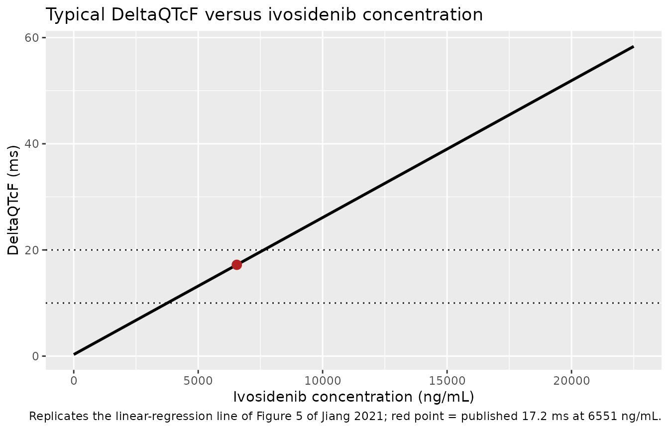
# Drive the C-QTc model with the simulated steady-state Cmax of each
# participant in the reference cohort.
ss_cmax <- nca_tab |>
  dplyr::filter(period == "Steady state", PPTESTCD == "cmax") |>
  dplyr::select(id, cmax = PPORRES)
ev_qt_cohort <- data.frame(id = ss_cmax$id, time = 0, evid = 0L,
                           CP_IVOSIDENIB_NGML = ss_cmax$cmax)
qt_cohort <- rxode2::rxSolve(mod_qt, events = ev_qt_cohort, returnType = "data.frame")
#> Warning: multi-subject simulation without without 'omega'
summary(qt_cohort$QTcF)
#>    Min. 1st Qu.  Median    Mean 3rd Qu.    Max.
#>   5.567   9.996  13.146  13.466  16.006  29.461
At the model-predicted typical steady-state Cmax of 4827 ng/mL the model gives about 12.8 ms. The paper’s 17.2 ms is evaluated at the observed geometric-mean Cmax of 6551 ng/mL, which is higher than the popPK typical-value Cmax (the paper does not say which studies or visits that geometric mean was taken from).
Assumptions and deviations
-
First-dose volumes in Table 1. The derived
first-dose rows for Vc/F, Q/F and Vp/F in Table 1 divide the
steady-state values by the full 3.3-fold apparent-clearance factor. The
text and Figure 1a change only
FrelandCL, and the printed single-dose half-life range falsifies the table’s volumes (see “How the first-dose step is encoded”). The packaged model follows the text and figure; it does not use those rows. -
Timing of the first-dose step. The paper does not
print the switching rule.
MULTI_DOSE_PTswitches at the second dose, following Supplementary Figure S1c (“the factors begin to influence the pharmacokinetic curve” at the start of once-daily dosing) and the Figure 1b grouping of the escalation day -3 dose with the expansion cycle 1 day 1 dose as the “first dose”. The switch is a step; the paper estimates no induction time course. -
Tlag as a zero-order release duration. The Table 1
footnote defines
Tlagas the “zero-order release duration (lag-time)”, and the base model is described as “sequential zero-order release (lag time) and first-order oral absorption”, so it is encoded asdur(depot). Dose records must carryrate = -2. -
Dose on relative bioavailability.
DOSEis the amount per administration with reference 500 mg (confirmed by Figure 2c). The paper does not say how the 100 mg twice-daily cohort (4 patients) was coded. - Albumin. The albumin ratio is time-varying albumin divided by baseline albumin (Table 1 footnote); the covariate cohort holds each participant’s ratio constant over time.
-
CYP3A4 inhibitors. The paper’s “other strong or
moderate CYP3A4 inhibitors” group excludes voriconazole, fluconazole and
posaconazole. The model forms it from
CONMED_CYP3A4_INH_MODandCONMED_CYP3A4_INH_STRONGand switches it off when any of the three azoles is flagged, so a record coded by inhibitor strength is not counted twice. The paper does not name the agents in the “other” or “mild” groups. - Between-subject variability. Table 1 reports CV% for CL/F, Vc/F and ka, and the footnote gives RSEs “on standard deviation terms”, so CV%/100 is taken as the SD of each eta (omega^2 = (CV%/100)^2). No correlations are reported; the etas are independent.
-
Residual error. “Log-additive CV% 26” is encoded as
lnorm(0.26). - C-QTc intercept, variability and covariates. Only the slope is printed. The intercept (0.30 ms) is back-solved from the printed prediction of 17.2 ms at 6551 ng/mL; because both printed numbers are rounded, it is uncertain by about +/- 0.1 ms. The between-subject variances of intercept and slope, the residual error and the intercept covariates (age, baseline QTcF, calcium, magnesium, QT-prolonging co-medication) are not reported, so the packaged C-QTc model is typical-value only with residual error set to 0.
- Exposure-response. The efficacy and safety analyses found no exposure relationship and produced no final model, and the logistic fits shown in Figure 4 have no printed coefficients, so none is packaged.
- Tmax. The simulated median Tmax (about 2.0 h after the first dose, 1.75 h at steady state) is slightly below the printed ranges of median Tmax by dose cohort, which come from sparse sampling in small escalation cohorts.
- Virtual cohorts. Covariate distributions are approximations of Tables S1 and S2 (normal/log-normal draws truncated to the observed ranges; one inhibitor category per participant).
- No correction notice for this article was found in Europe PMC as of 2026-09-28.