Valproic acid in paediatric and adult Caucasian patients (Teixeira-da-Silva 2022)
Source:vignettes/articles/TeixeiradaSilva_2022_valproic_acid.Rmd
TeixeiradaSilva_2022_valproic_acid.RmdModel and source
Teixeira-da-Silva et al. (2022) developed a one-compartment population pharmacokinetic model with first-order absorption and elimination for total serum valproic acid (VPA). The data were 1751 routine therapeutic-drug-monitoring (TDM) samples from 836 Spanish outpatients aged 0.11 to 89.4 years, 97.5% of them steady-state troughs. Because troughs carry almost no information about absorption or distribution, the authors fixed the formulation-specific absorption rate constants and the apparent volume from the literature and estimated only apparent clearance and its covariates:
PHT, PB and CBZ are 1 when
phenytoin, phenobarbital or carbamazepine is given with VPA and 0
otherwise. Ka is fixed at 2.64 1/h for the oral solution,
0.78 1/h for gastro-resistant tablets and 0.38 1/h for modified-release
coated tablets.
mod <- rxode2::rxode(readModelDb("TeixeiradaSilva_2022_valproic_acid"))
#> ℹ parameter labels from comments will be replaced by 'label()'
mod_ui <- mod
mod
#>  ── rxode2-based free-form 2-cmt ODE model ──────────────────────────────────────
#>  ── Initalization: ──
#> Fixed Effects ($theta):
#>              lka e_form_tablet_ka e_form_vpa_sr_ka              lcl
#>        0.9707789       -1.2192403       -1.9383629       -0.4369558
#>              lvc          e_wt_cl          e_wt_vc         e_age_cl
#>        2.6390573        0.7500000        1.0000000       -0.0154000
#>  e_conmed_pht_cl   e_conmed_pb_cl  e_conmed_cbz_cl            expSd
#>        0.6400000        0.3860000        0.5210000        0.2757000
#>
#> Omega ($omega):
#>         etalcl
#> etalcl 0.06938
#> attr(,"lotriLabels")
#> [1] "Table 2 row 'IIV_CL/F (%)' = 26.8 (RSE 5.50%, shrinkage 19.0%); bootstrap median 26.6"
#> attr(,"lotriFix")
#>        etalcl
#> etalcl  FALSE
#>
#> States ($state or $stateDf):
#>   Compartment Number Compartment Name
#> 1                  1            depot
#> 2                  2          central
#>  ── μ-referencing ($muRefTable): ──
#>   theta    eta level
#> 1   lcl etalcl    id
#>                                                                      covariates
#> 1 log(0.0142857142857143 * WT)*e_wt_cl + log(0.0666666666666667 * AGE)*e_age_cl
#>
#>  ── Model (Normalized Syntax): ──
#> function() {
#>     compartmentData <- list(depot = list(analyte = "valproic acid",
#>         units = "mg", specimen = "administration site", verified = TRUE),
#>         central = list(analyte = "valproic acid", units = "mg",
#>             specimen = "serum", verified = TRUE))
#>     covariateData <- list(WT = list(description = "Total body weight",
#>         units = "kg", type = "continuous", reference_category = "70 kg (Equations (1) and (2))",
#>         notes = "Allometric scaling fixed a priori: exponent 0.75 on CL/F and 1 on V/F, both normalised to 70 kg (Methods 2.3; Supplementary Table S2 'TVCL = THETA(1) * (TBW/70)**0.75', 'TVV = THETA(2) * (TBW/70)**1'). Development cohort 6.70-125.00 kg, median 60.00 kg (Table 1).",
#>         source_name = "TBW"), AGE = list(description = "Age",
#>         units = "years", type = "continuous", reference_category = "15 years (Equation (1))",
#>         notes = "Power effect on CL/F centred on 15 years, (AGE/15)^-0.0154 (Equation (1); Supplementary Table S2 'CLAGE = ((AGE/15)**THETA(3))'). The centring value is the cut-off the authors saw on a plot of CL/F against age (Results 3.1). The exponent is imprecise (64.3% RSE; bootstrap 95% CI -0.034 to 0.004 crosses zero), and its effect is small: about +4% at 1 year and -1% at 35 years. Development cohort 0.11-89.42 years (Table 1).",
#>         source_name = "AGE"), CONMED_PHT = list(description = "Concomitant phenytoin indicator",
#>         units = "(binary)", type = "binary", reference_category = "0 (no concomitant phenytoin)",
#>         notes = "Proportional effect on CL/F, (1 + 0.640)^PHT = 1.640 (Equation (1); Supplementary Table S2 'CLPHT = ( 1 + THETA(6))'). 18 of 836 development patients (39 samples) received phenytoin (Supplementary Table S1). Only mono- or dual therapy was admitted, so the three inducer indicators are mutually exclusive in the source data.",
#>         source_name = "PHT"), CONMED_PB = list(description = "Concomitant phenobarbital indicator",
#>         units = "(binary)", type = "binary", reference_category = "0 (no concomitant phenobarbital)",
#>         notes = "Proportional effect on CL/F, (1 + 0.386)^PB = 1.386 (Equation (1); Supplementary Table S2 'CLPB = ( 1 + THETA(5))'). 19 of 836 development patients (37 samples) received phenobarbital (Supplementary Table S1).",
#>         source_name = "PB"), CONMED_CBZ = list(description = "Concomitant carbamazepine indicator",
#>         units = "(binary)", type = "binary", reference_category = "0 (no concomitant carbamazepine)",
#>         notes = "Proportional effect on CL/F, (1 + 0.521)^CBZ = 1.521 (Equation (1); Supplementary Table S2 'CLCBZ = ( 1 + THETA(4))'). Table 2 prints the coefficient as 0.512, a transposition of the 0.521 that Equation (1) and the Discussion ('an increase CL/F of about 52%', and CL/F ratios of 0.818 / 0.538 = 1.520 and 2.258 / 1.484 = 1.522) both use; the equation value is encoded. 58 of 836 development patients (139 samples) received carbamazepine (Supplementary Table S1).",
#>         source_name = "CBZ"), FORM_TABLET = list(description = "Gastro-resistant (enteric-coated) valproic acid tablet indicator",
#>         units = "(binary)", type = "binary", reference_category = "0 (oral solution / syrup, Ka = 2.64 1/h)",
#>         notes = "Selects the FIXED gastro-resistant-tablet absorption rate constant Ka = 0.78 1/h (Methods 2.3 and Table 2 footnote; Supplementary Table S2 'IF (FFS.EQ.2) KA=0.78'). The source FFS column is four-level {0 = not available, 1 = oral solution, 2 = gastro-resistant tablet, 3 = modified-release coated tablet}; FFS = 0 was also given Ka = 0.78, so a record with unknown formulation maps to FORM_TABLET = 1. Methods 2.3 states that missing formulation information was imputed as oral solution below 12 years of age and gastro-resistant tablet from 12 years. Pairs with FORM_VPA_SR; both 0 = oral solution.",
#>         source_name = "FFS"), FORM_VPA_SR = list(description = "Modified-release (prolonged-release) coated valproic acid tablet indicator",
#>         units = "(binary)", type = "binary", reference_category = "0 (oral solution / syrup, Ka = 2.64 1/h)",
#>         notes = "Selects the FIXED modified-release-coated-tablet absorption rate constant Ka = 0.38 1/h (Methods 2.3 and Table 2 footnote; Supplementary Table S2 'IF (FFS.EQ.3) KA=0.38'). Available presentations were 300 mg and 500 mg coated prolonged-release tablets (Methods 2.2). Set FORM_TABLET = 0 when FORM_VPA_SR = 1.",
#>         source_name = "FFS"))
#>     covariatesDataExcluded <- list(SEXF = list(description = "Female sex indicator",
#>         units = "(binary)", type = "binary", notes = "Statistically significant on CL/F in the stepwise forward step (p < 0.005) but not retained in the final model because it changed CL/F by less than 10% (Results 3.1); no coefficient is reported. 385 of 836 development patients (46.1%) were female (Table 1).",
#>         source_name = "SEX"), CONMED_LAMOTRIGINE = list(description = "Concomitant lamotrigine indicator",
#>         units = "(binary)", type = "binary", notes = "Statistically significant on CL/F in the stepwise forward step (p < 0.005) but not retained because it changed CL/F by less than 10% (Results 3.1 and Discussion); no coefficient is reported. 50 of 836 development patients received lamotrigine (Supplementary Table S1).",
#>         source_name = "LTG"))
#>     description <- "One-compartment population PK model with first-order absorption for total serum valproic acid in Caucasian (Spanish) paediatric and adult outpatients followed by therapeutic drug monitoring (Teixeira-da-Silva 2022 final model). Apparent clearance scales allometrically with total body weight (fixed exponent 0.75), carries a small power effect of age centred on 15 years, and is increased by concomitant phenytoin (x1.640), phenobarbital (x1.386) and carbamazepine (x1.521). Apparent volume is fixed at 14 L per 70 kg (linear in weight) and the formulation-specific absorption rate constants are fixed from the literature (oral solution 2.64, gastro-resistant tablet 0.78, modified-release coated tablet 0.38 1/h)."
#>     population <- list(species = "human", n_subjects = 836, n_studies = 1,
#>         n_observations = 1751, age_range = "0.11-89.42 years",
#>         age_median = "32.42 years", weight_range = "6.70-125.00 kg",
#>         weight_median = "60.00 kg", sex_female_pct = 46.1, race_ethnicity = "Caucasian (Spanish)",
#>         disease_state = "Outpatients receiving valproic acid (epilepsy and other neurological or psychiatric indications) in mono- or dual antiepileptic therapy",
#>         dose_range = "150-4500 mg/day (median 1000 mg/day); oral solution 200 mg/mL, gastro-resistant tablets 200 and 500 mg, prolonged-release coated tablets 300 and 500 mg",
#>         regions = "Spain (therapeutic drug monitoring programme, University Hospital of Salamanca)",
#>         co_medication = "Development dataset: carbamazepine 58, phenytoin 18, phenobarbital 19, lamotrigine 50, topiramate 13, ethosuximide 3, clobazam 8, primidone 1, other dual therapies 280 patients (Supplementary Table S1). At most one antiepileptic in addition to valproic acid.",
#>         age_groups = "Development dataset by age: 28 days-2 years 33 patients (47 samples), 2-11 years 208 (419), 12-18 years 70 (157), > 18 years 525 (1128) (Supplementary Table S1)",
#>         notes = "Development dataset of 836 patients and 1751 serum samples (Table 1 and Supplementary Table S1; the Abstract says 776 patients, which is the external-evaluation sample count). External evaluation dataset of 368 patients and 776 samples. 97.5% of samples were steady-state troughs from routine therapeutic drug monitoring, measured by fluorescence polarisation immunoassay (Abbott TDx). Fitted in NONMEM 7.5.1 with FOCEI and log-transform-both-sides. Patients with BMI outside 16.0-39.9 kg/m2 were excluded.")
#>     reference <- "Teixeira-da-Silva P, Perez-Blanco JS, Santos-Buelga D, Otero MJ, Garcia MJ. Population Pharmacokinetics of Valproic Acid in Pediatric and Adult Caucasian Patients. Pharmaceutics. 2022;14(4):811. doi:10.3390/pharmaceutics14040811. PMCID PMC9031051. Final-model estimates from Table 2 (development dataset) and Equations (1)-(2); model structure from the NONMEM control stream in Supplementary Table S2."
#>     units <- list(time = "h", dosing = "mg", concentration = "mg/L")
#>     vignette <- "TeixeiradaSilva_2022_valproic_acid"
#>     ini({
#>         lka <- fix(0.970778917158225)
#>         label("Absorption rate constant, oral solution reference (1/h)")
#>         e_form_tablet_ka <- fix(-1.21924027645672)
#>         label("Log-ratio shift on Ka for gastro-resistant tablet vs oral solution")
#>         e_form_vpa_sr_ka <- fix(-1.93836294341993)
#>         label("Log-ratio shift on Ka for modified-release coated tablet vs oral solution")
#>         lcl <- -0.436955775199535
#>         label("Apparent clearance CL/F for a 70 kg, 15-year-old patient on monotherapy (L/h)")
#>         lvc <- fix(2.63905732961526)
#>         label("Apparent volume of distribution V/F for a 70 kg patient (L)")
#>         e_wt_cl <- fix(0.75)
#>         label("Allometric exponent on (WT/70) for CL/F (unitless)")
#>         e_wt_vc <- fix(1)
#>         label("Allometric exponent on (WT/70) for V/F (unitless)")
#>         e_age_cl <- -0.0154
#>         label("Power exponent on (AGE/15) for CL/F (unitless)")
#>         e_conmed_pht_cl <- 0.64
#>         label("Fractional increase in CL/F with concomitant phenytoin (unitless)")
#>         e_conmed_pb_cl <- 0.386
#>         label("Fractional increase in CL/F with concomitant phenobarbital (unitless)")
#>         e_conmed_cbz_cl <- 0.521
#>         label("Fractional increase in CL/F with concomitant carbamazepine (unitless)")
#>         expSd <- c(0, 0.2757)
#>         label("Residual SD on the log scale (log-transform-both-sides)")
#>         etalcl ~ 0.06938
#>         label("Table 2 row 'IIV_CL/F (%)' = 26.8 (RSE 5.50%, shrinkage 19.0%); bootstrap median 26.6")
#>     })
#>     model({
#>         ka <- exp(lka + e_form_tablet_ka * FORM_TABLET + e_form_vpa_sr_ka *
#>             FORM_VPA_SR)
#>         cl <- exp(lcl + e_wt_cl * log(WT/70) + e_age_cl * log(AGE/15) +
#>             etalcl) * (1 + e_conmed_pht_cl * CONMED_PHT) * (1 +
#>             e_conmed_pb_cl * CONMED_PB) * (1 + e_conmed_cbz_cl *
#>             CONMED_CBZ)
#>         vc <- exp(lvc + e_wt_vc * log(WT/70))
#>         kel <- cl/vc
#>         d/dt(depot) <- -ka * depot
#>         d/dt(central) <- ka * depot - kel * central
#>         Cc <- central/vc
#>         Cc ~ lnorm(expSd)
#>     })
#> }
Population
| Field | Value |
|---|---|
| species | human |
| n_subjects | 836 |
| n_studies | 1 |
| n_observations | 1751 |
| age_range | 0.11-89.42 years |
| age_median | 32.42 years |
| weight_range | 6.70-125.00 kg |
| weight_median | 60.00 kg |
| sex_female_pct | 46.1 |
| race_ethnicity | Caucasian (Spanish) |
| disease_state | Outpatients receiving valproic acid (epilepsy and other neurological or psychiatric indications) in mono- or dual antiepileptic therapy |
| dose_range | 150-4500 mg/day (median 1000 mg/day); oral solution 200 mg/mL, gastro-resistant tablets 200 and 500 mg, prolonged-release coated tablets 300 and 500 mg |
| regions | Spain (therapeutic drug monitoring programme, University Hospital of Salamanca) |
| co_medication | Development dataset: carbamazepine 58, phenytoin 18, phenobarbital 19, lamotrigine 50, topiramate 13, ethosuximide 3, clobazam 8, primidone 1, other dual therapies 280 patients (Supplementary Table S1). At most one antiepileptic in addition to valproic acid. |
| age_groups | Development dataset by age: 28 days-2 years 33 patients (47 samples), 2-11 years 208 (419), 12-18 years 70 (157), > 18 years 525 (1128) (Supplementary Table S1) |
| notes | Development dataset of 836 patients and 1751 serum samples (Table 1 and Supplementary Table S1; the Abstract says 776 patients, which is the external-evaluation sample count). External evaluation dataset of 368 patients and 776 samples. 97.5% of samples were steady-state troughs from routine therapeutic drug monitoring, measured by fluorescence polarisation immunoassay (Abbott TDx). Fitted in NONMEM 7.5.1 with FOCEI and log-transform-both-sides. Patients with BMI outside 16.0-39.9 kg/m2 were excluded. |
The cohort spans more than three orders of magnitude of age: 33 infants (28 days to 2 years), 208 children (2-11 years), 70 adolescents and 525 adults. Enzyme-inducing comedication is uncommon but was highly influential: 58 patients received carbamazepine, 18 phenytoin and 19 phenobarbital. Only mono- or dual therapy was admitted, so no patient received more than one of the three.
Source trace
| Quantity | Value | Source |
|---|---|---|
| Structural model | 1-compartment, first-order absorption and elimination | Methods 2.3; Results 3.1; Supplementary Table S2 (ADVAN2 TRANS2) |
| ODE: depot | d/dt(depot) = -ka * depot | Supplementary Table S2 (ADVAN2) |
| ODE: central | d/dt(central) = ka * depot - (CL/V) * central | Supplementary Table S2 (ADVAN2, K = CL/V) |
| Observation | Cc = central / V (mg/L) | Supplementary Table S2 (SC = V) |
| Ka, oral solution | 2.64 1/h, fixed | Methods 2.3; Table 2 footnote; Supplementary Table S2 (FFS = 1) |
| Ka, gastro-resistant tablet | 0.78 1/h, fixed | Methods 2.3; Table 2 footnote; Supplementary Table S2 (FFS = 0 and 2) |
| Ka, modified-release coated tablet | 0.38 1/h, fixed | Methods 2.3; Table 2 footnote; Supplementary Table S2 (FFS = 3) |
| CL/F, 70 kg, 15 y, monotherapy | 0.646 L/h | Table 2 (RSE 1.20%); Equation (1) |
| V/F, 70 kg | 14 L, fixed | Table 2 footnote; Equation (2); Supplementary Table S2 (‘14 FIX’) |
| Weight exponent on CL/F | 0.75, fixed | Methods 2.3; Equation (1) |
| Weight exponent on V/F | 1, fixed | Methods 2.3; Equation (2) |
| Age exponent on CL/F (AGE/15) | -0.0154 | Table 2 (RSE 64.3%); Equation (1) |
| Phenytoin on CL/F | x (1 + 0.640) = 1.640 | Table 2 (RSE 24.2%); Equation (1) |
| Phenobarbital on CL/F | x (1 + 0.386) = 1.386 | Table 2 (RSE 23.2%); Equation (1) |
| Carbamazepine on CL/F | x (1 + 0.521) = 1.521 | Equation (1); Discussion ‘about 52%’ (Table 2 prints 0.512) |
| IIV on CL/F | 26.8% CV -> omega^2 = log(0.268^2 + 1) = 0.06938 | Table 2 (RSE 5.50%, shrinkage 19.0%) |
| IIV on V/F | fixed to 0 (omitted) | Supplementary Table S2 (‘$OMEGA … 0 FIX’) |
| Residual error | additive on log scale (LTBS), 28.1% -> expSd = 0.2757 | Methods 2.3; Supplementary Table S2; Table 2 bootstrap median (see below) |
Verification
Covariate multipliers against Equation (1) and the Discussion
The comedication effects are coded in the control stream as
(1 + THETA) when the drug is present. Equation (1) prints
the resulting factors, and the Discussion quotes each one again as a
percent increase in CL/F and as ratios of typical-patient
clearances.
ini_vals <- mod_ui$theta
mult <- tibble::tibble(
  Comedication = c("Phenytoin", "Phenobarbital", "Carbamazepine"),
  `Model factor` = 1 + unname(ini_vals[c("e_conmed_pht_cl", "e_conmed_pb_cl", "e_conmed_cbz_cl")]),
  `Equation (1)` = c(1.640, 1.386, 1.521),
  `Discussion ratio` = c(0.883 / 0.538, 0.746 / 0.538, 0.818 / 0.538),
  `Discussion prose` = c("about 64%", "about 39%", "about 52%")
)
knitr::kable(mult, digits = 3, caption = "Comedication multipliers on CL/F.")| Comedication | Model factor | Equation (1) | Discussion ratio | Discussion prose |
|---|---|---|---|---|
| Phenytoin | 1.640 | 1.640 | 1.641 | about 64% |
| Phenobarbital | 1.386 | 1.386 | 1.387 | about 39% |
| Carbamazepine | 1.521 | 1.521 | 1.520 | about 52% |
stopifnot(
  all(abs(mult$`Model factor` - mult$`Equation (1)`) < 1e-9),
  all(abs(mult$`Model factor` - mult$`Discussion ratio`) < 0.005)
)
For carbamazepine, Table 2 prints the coefficient as 0.512, which would give a factor of 1.512. Equation (1) prints 1.521, the Discussion says “about 52%”, and both of its carbamazepine-to-monotherapy clearance ratios (0.818 / 0.538 = 1.520 and 2.258 / 1.484 = 1.522) agree with 1.521. The Table 2 entry is read as a transposition of 0.521. The two readings differ by 0.6% in clearance.
Typical-patient closed form
Equation (1) and Equation (2) evaluated directly must match the
model’s individual cl and vc for a
typical-value solve.
typ_cov <- function(age, wt, pht = 0, pb = 0, cbz = 0, tab = 0, sr = 0) {
  data.frame(AGE = age, WT = wt, CONMED_PHT = pht, CONMED_PB = pb,
             CONMED_CBZ = cbz, FORM_TABLET = tab, FORM_VPA_SR = sr)
}
eq1 <- function(age, wt, pht = 0, pb = 0, cbz = 0) {
  0.646 * (wt / 70)^0.75 * 1.640^pht * 1.386^pb * 1.521^cbz * (age / 15)^-0.0154
}

check_pts <- tibble::tibble(age = c(1, 6, 15, 35, 70), wt = c(10, 21, 56, 70, 80))
ev1 <- rxode2::et(amt = 500, cmt = "depot") |> rxode2::et(c(0, 1), cmt = "central")
closed <- check_pts |>
  rowwise() |>
  mutate(
    sim = list(rxode2::rxSolve(mod, cbind(as.data.frame(ev1), typ_cov(age, wt)),
                               omega = NA, returnType = "data.frame")),
    cl_model = sim$cl[1], vc_model = sim$vc[1],
    cl_eq1 = eq1(age, wt), vc_eq2 = 14 * wt / 70
  ) |>
  ungroup() |>
  select(-sim)
knitr::kable(closed, digits = 4, caption = "Model CL/F and V/F against Equations (1) and (2).")| age | wt | cl_model | vc_model | cl_eq1 | vc_eq2 |
|---|---|---|---|---|---|
| 1 | 10 | 0.1565 | 2.0 | 0.1565 | 2.0 |
| 6 | 21 | 0.2656 | 4.2 | 0.2656 | 4.2 |
| 15 | 56 | 0.5464 | 11.2 | 0.5464 | 11.2 |
| 35 | 70 | 0.6376 | 14.0 | 0.6376 | 14.0 |
| 70 | 80 | 0.6973 | 16.0 | 0.6973 | 16.0 |
Replicating Figure 2
Figure 2 of the paper shows typical-patient steady-state profiles over one dosing interval for four patients (1 y / 10 kg, 6 y / 21 kg, 15 y / 56 kg and 35 y / 70 kg), each on monotherapy and with each of the three inducers. The maintainers digitised the peak and the end-of-interval trough of every curve from the figure; peaks and troughs are read to about +/- 1.5 mg/L.
panels <- tibble::tribble(
  ~panel,                                        ~age, ~wt, ~dose, ~tau, ~tab,
  "1 y; 10 kg; 100 mg q8h (oral solution)",          1,  10,   100,    8,    0,
  "6 y; 21 kg; 200 mg q8h (oral solution)",          6,  21,   200,    8,    0,
  "15 y; 56 kg; 1000 mg q24h (GR tablet)",          15,  56,  1000,   24,    1,
  "35 y; 70 kg; 1200 mg q24h (GR tablet)",          35,  70,  1200,   24,    1
)
regimens <- tibble::tribble(
  ~therapy,                    ~pht, ~pb, ~cbz,
  "Monotherapy",                  0,   0,    0,
  "Dual therapy with PHT",        1,   0,    0,
  "Dual therapy with PB",         0,   1,    0,
  "Dual therapy with CBZ",        0,   0,    1
)
scen <- tidyr::crossing(panels, regimens) |>
  mutate(scenario = paste(panel, therapy, sep = " | "), id = row_number())

fig2_events <- bind_rows(lapply(seq_len(nrow(scen)), function(i) {
  s <- scen[i, ]
  ev <- rxode2::et(amt = s$dose, ii = s$tau, ss = 1, cmt = "depot") |>
    rxode2::et(seq(0, s$tau, by = 0.05), cmt = "central")
  cbind(as.data.frame(ev) |> select(-any_of("id")),
        typ_cov(s$age, s$wt, s$pht, s$pb, s$cbz, s$tab)) |>
    mutate(id = s$id)
}))
fig2 <- rxode2::rxSolve(mod, fig2_events, omega = NA, returnType = "data.frame") |>
  left_join(scen |> select(id, panel, therapy, scenario, tau), by = "id")
#> Warning: multi-subject simulation without without 'omega'
digitised <- tibble::tribble(
  ~panel,                                       ~therapy,                ~cmax, ~cmin,
  "1 y; 10 kg; 100 mg q8h (oral solution)",     "Monotherapy",            98.4,  59.1,
  "1 y; 10 kg; 100 mg q8h (oral solution)",     "Dual therapy with PHT",  68.4,  29.4,
  "1 y; 10 kg; 100 mg q8h (oral solution)",     "Dual therapy with PB",   77.0,  37.7,
  "1 y; 10 kg; 100 mg q8h (oral solution)",     "Dual therapy with CBZ",  72.1,  35.9,
  "6 y; 21 kg; 200 mg q8h (oral solution)",     "Monotherapy",            93.1,  55.7,
  "6 y; 21 kg; 200 mg q8h (oral solution)",     "Dual therapy with PHT",  64.0,  27.5,
  "6 y; 21 kg; 200 mg q8h (oral solution)",     "Dual therapy with PB",   73.0,  35.3,
  "6 y; 21 kg; 200 mg q8h (oral solution)",     "Dual therapy with CBZ",  68.4,  33.7,
  "15 y; 56 kg; 1000 mg q24h (GR tablet)",      "Monotherapy",           110.0,  42.5,
  "15 y; 56 kg; 1000 mg q24h (GR tablet)",      "Dual therapy with PHT",  82.1,  16.1,
  "15 y; 56 kg; 1000 mg q24h (GR tablet)",      "Dual therapy with PB",   90.0,  23.6,
  "15 y; 56 kg; 1000 mg q24h (GR tablet)",      "Dual therapy with CBZ",  85.2,  19.2,
  "35 y; 70 kg; 1200 mg q24h (GR tablet)",      "Monotherapy",           111.0,  45.9,
  "35 y; 70 kg; 1200 mg q24h (GR tablet)",      "Dual therapy with PHT",  81.5,  18.3,
  "35 y; 70 kg; 1200 mg q24h (GR tablet)",      "Dual therapy with PB",   90.0,  25.7,
  "35 y; 70 kg; 1200 mg q24h (GR tablet)",      "Dual therapy with CBZ",  85.2,  21.7
) |>
  mutate(scenario = paste(panel, therapy, sep = " | "))

pal <- c("Monotherapy" = "#5B9BD5", "Dual therapy with PHT" = "#ED7D31",
         "Dual therapy with PB" = "#A5A5A5", "Dual therapy with CBZ" = "#FFC000")
dig_pts <- digitised |>
  left_join(panels |> select(panel, tau), by = "panel") |>
  tidyr::pivot_longer(c(cmax, cmin), names_to = "stat", values_to = "Cc") |>
  left_join(fig2 |> group_by(scenario) |> summarise(tmax = time[which.max(Cc)]), by = "scenario") |>
  mutate(time = ifelse(stat == "cmax", tmax, tau))

ggplot(fig2, aes(time, Cc, colour = therapy)) +
  geom_line(linewidth = 0.8) +
  geom_point(data = dig_pts, shape = 21, fill = "white", size = 2) +
  facet_wrap(~panel, scales = "free_x") +
  scale_colour_manual(values = pal) +
  coord_cartesian(ylim = c(0, 150)) +
  labs(x = "Time since last dose (h)", y = "VPA concentration (mg/L)", colour = NULL) +
  theme_bw() +
  theme(legend.position = "bottom")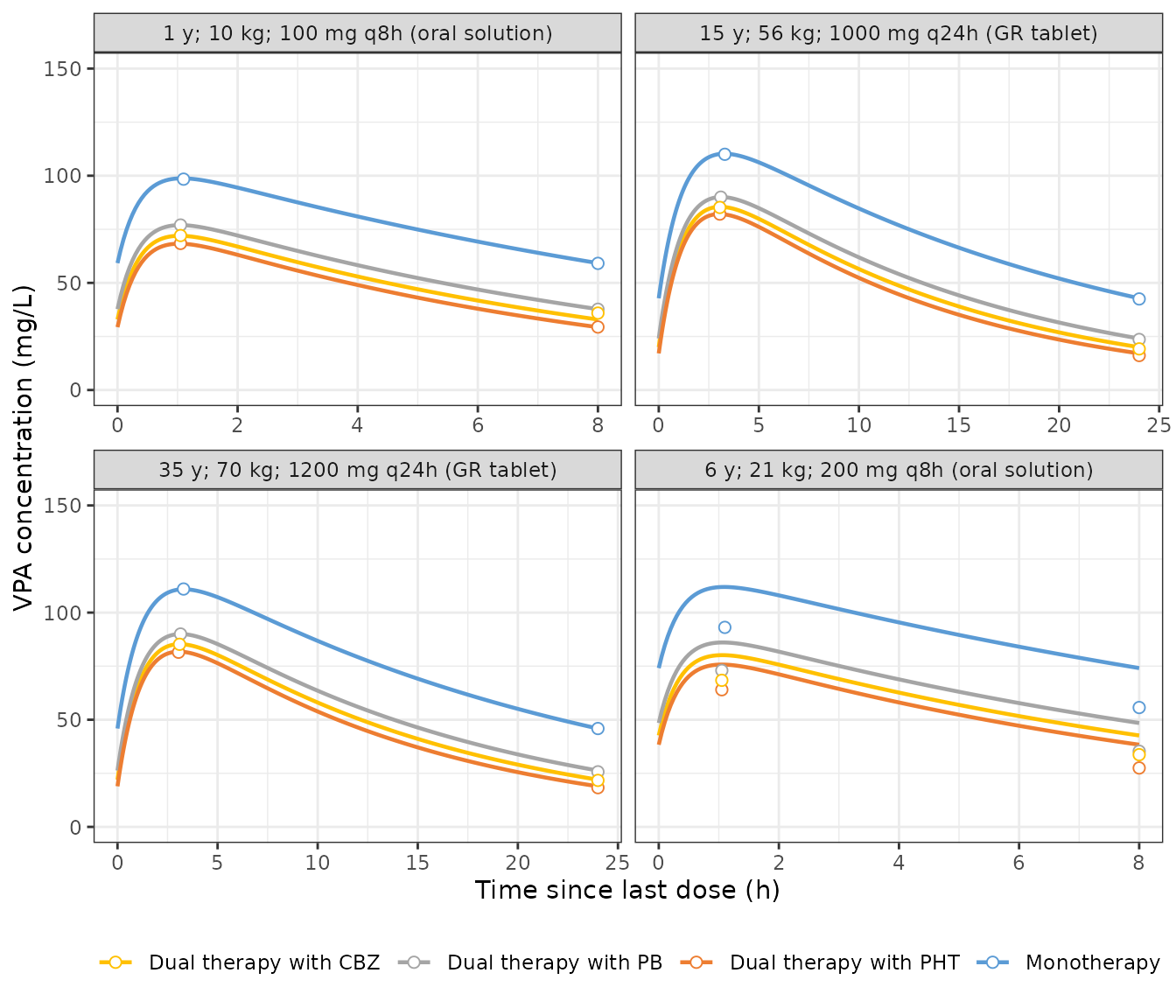
Replicates Figure 2 of Teixeira-da-Silva 2022: typical-patient steady-state VPA profiles over one dosing interval. Points are the peaks and troughs digitised from the published figure.
PKNCA on the Figure 2 profiles
fig2_conc <- fig2 |>
  filter(!is.na(Cc)) |>
  select(scenario, id, time, Cc)
fig2_dose <- fig2_events |>
  filter(evid == 1) |>
  left_join(scen |> select(id, scenario), by = "id") |>
  select(scenario, id, time, amt)
fig2_int <- scen |>
  transmute(scenario, id, start = 0, end = tau, cmax = TRUE, cmin = TRUE, cav = TRUE)

fig2_nca <- PKNCA::pk.nca(PKNCA::PKNCAdata(
  PKNCA::PKNCAconc(fig2_conc, Cc ~ time | scenario + id, concu = "mg/L", timeu = "h"),
  PKNCA::PKNCAdose(fig2_dose, amt ~ time | scenario + id, doseu = "mg"),
  intervals = fig2_int
))

sim_wide <- as.data.frame(fig2_nca$result) |>
  filter(PPTESTCD %in% c("cmax", "cmin")) |>
  select(scenario, PPTESTCD, PPORRES) |>
  tidyr::pivot_wider(names_from = PPTESTCD, values_from = PPORRES)

nlmixr2lib::ncaComparisonTable(
  simulated = sim_wide,
  reference = digitised |> select(scenario, cmax, cmin),
  by = "scenario",
  units = c(cmax = "mg/L", cmin = "mg/L")
) |>
knitr::kable(caption = "Simulated steady-state Cmax and Cmin against values digitised from Figure 2. * differs by more than 20%.")| NCA parameter | scenario | Reference | Simulated | % diff |
|---|---|---|---|---|
| Cmax (mg/L) | 1 y; 10 kg; 100 mg q8h (oral solution) | Monotherapy | 98.4 | 98.8 | +0.4% |
| Cmax (mg/L) | 1 y; 10 kg; 100 mg q8h (oral solution) | Dual therapy with PHT | 68.4 | 68.3 | -0.2% |
| Cmax (mg/L) | 1 y; 10 kg; 100 mg q8h (oral solution) | Dual therapy with PB | 77 | 77 | -0.1% |
| Cmax (mg/L) | 1 y; 10 kg; 100 mg q8h (oral solution) | Dual therapy with CBZ | 72.1 | 72 | -0.2% |
| Cmax (mg/L) | 6 y; 21 kg; 200 mg q8h (oral solution) | Monotherapy | 93.1 | 112 | +20.3%* |
| Cmax (mg/L) | 6 y; 21 kg; 200 mg q8h (oral solution) | Dual therapy with PHT | 64 | 75.7 | +18.4% |
| Cmax (mg/L) | 6 y; 21 kg; 200 mg q8h (oral solution) | Dual therapy with PB | 73 | 86.1 | +17.9% |
| Cmax (mg/L) | 6 y; 21 kg; 200 mg q8h (oral solution) | Dual therapy with CBZ | 68.4 | 80.1 | +17.2% |
| Cmax (mg/L) | 15 y; 56 kg; 1000 mg q24h (GR tablet) | Monotherapy | 110 | 110 | +0.2% |
| Cmax (mg/L) | 15 y; 56 kg; 1000 mg q24h (GR tablet) | Dual therapy with PHT | 82.1 | 82.1 | +0.0% |
| Cmax (mg/L) | 15 y; 56 kg; 1000 mg q24h (GR tablet) | Dual therapy with PB | 90 | 90 | +0.1% |
| Cmax (mg/L) | 15 y; 56 kg; 1000 mg q24h (GR tablet) | Dual therapy with CBZ | 85.2 | 85.5 | +0.3% |
| Cmax (mg/L) | 35 y; 70 kg; 1200 mg q24h (GR tablet) | Monotherapy | 111 | 111 | -0.1% |
| Cmax (mg/L) | 35 y; 70 kg; 1200 mg q24h (GR tablet) | Dual therapy with PHT | 81.5 | 81.8 | +0.3% |
| Cmax (mg/L) | 35 y; 70 kg; 1200 mg q24h (GR tablet) | Dual therapy with PB | 90 | 90 | -0.0% |
| Cmax (mg/L) | 35 y; 70 kg; 1200 mg q24h (GR tablet) | Dual therapy with CBZ | 85.2 | 85.3 | +0.1% |
| Cmin (mg/L) | 1 y; 10 kg; 100 mg q8h (oral solution) | Monotherapy | 59.1 | 59.2 | +0.2% |
| Cmin (mg/L) | 1 y; 10 kg; 100 mg q8h (oral solution) | Dual therapy with PHT | 29.4 | 29.3 | -0.2% |
| Cmin (mg/L) | 1 y; 10 kg; 100 mg q8h (oral solution) | Dual therapy with PB | 37.7 | 37.7 | +0.1% |
| Cmin (mg/L) | 1 y; 10 kg; 100 mg q8h (oral solution) | Dual therapy with CBZ | 35.9 | 32.9 | -8.3% |
| Cmin (mg/L) | 6 y; 21 kg; 200 mg q8h (oral solution) | Monotherapy | 55.7 | 74.1 | +33.0%* |
| Cmin (mg/L) | 6 y; 21 kg; 200 mg q8h (oral solution) | Dual therapy with PHT | 27.5 | 38.3 | +39.5%* |
| Cmin (mg/L) | 6 y; 21 kg; 200 mg q8h (oral solution) | Dual therapy with PB | 35.3 | 48.5 | +37.3%* |
| Cmin (mg/L) | 6 y; 21 kg; 200 mg q8h (oral solution) | Dual therapy with CBZ | 33.7 | 42.7 | +26.6%* |
| Cmin (mg/L) | 15 y; 56 kg; 1000 mg q24h (GR tablet) | Monotherapy | 42.5 | 42.8 | +0.7% |
| Cmin (mg/L) | 15 y; 56 kg; 1000 mg q24h (GR tablet) | Dual therapy with PHT | 16.1 | 17.1 | +6.1% |
| Cmin (mg/L) | 15 y; 56 kg; 1000 mg q24h (GR tablet) | Dual therapy with PB | 23.6 | 24 | +1.8% |
| Cmin (mg/L) | 15 y; 56 kg; 1000 mg q24h (GR tablet) | Dual therapy with CBZ | 19.2 | 20 | +4.1% |
| Cmin (mg/L) | 35 y; 70 kg; 1200 mg q24h (GR tablet) | Monotherapy | 45.9 | 45.9 | -0.0% |
| Cmin (mg/L) | 35 y; 70 kg; 1200 mg q24h (GR tablet) | Dual therapy with PHT | 18.3 | 18.9 | +3.5% |
| Cmin (mg/L) | 35 y; 70 kg; 1200 mg q24h (GR tablet) | Dual therapy with PB | 25.7 | 26.3 | +2.2% |
| Cmin (mg/L) | 35 y; 70 kg; 1200 mg q24h (GR tablet) | Dual therapy with CBZ | 21.7 | 22 | +1.5% |
fig2_cmp <- sim_wide |>
  inner_join(digitised |> select(scenario, panel, cmax_pub = cmax, cmin_pub = cmin), by = "scenario") |>
  mutate(pct_cmax = 100 * (cmax - cmax_pub) / cmax_pub,
         pct_cmin = 100 * (cmin - cmin_pub) / cmin_pub)

fig2_cmp |>
  group_by(panel) |>
  summarise(`median Cmax diff (%)` = median(pct_cmax),
            `median Cmin diff (%)` = median(pct_cmin), .groups = "drop") |>
knitr::kable(digits = 1, caption = "Per-panel median difference, simulation vs Figure 2.")| panel | median Cmax diff (%) | median Cmin diff (%) |
|---|---|---|
| 1 y; 10 kg; 100 mg q8h (oral solution) | -0.1 | -0.1 |
| 15 y; 56 kg; 1000 mg q24h (GR tablet) | 0.1 | 3.0 |
| 35 y; 70 kg; 1200 mg q24h (GR tablet) | 0.0 | 1.8 |
| 6 y; 21 kg; 200 mg q8h (oral solution) | 18.1 | 35.2 |
# Panels 1, 3 and 4 reproduce Figure 2; panel 2 does not (see Errata).
ok <- fig2_cmp |> filter(!grepl("^6 y", panel))
stopifnot(
  abs(median(ok$pct_cmax)) < 3,
  quantile(abs(ok$pct_cmax), 0.9) < 5,
  abs(median(ok$pct_cmin)) < 5,
  quantile(abs(ok$pct_cmin), 0.9) < 12
)
Three of the four panels reproduce the published figure: peaks agree within about 1% and troughs within a few mg/L. The 1-year and 35-year monotherapy curves and the adolescent and adult dual-therapy curves agree to within the precision of digitising. The largest gap in those three panels is the 1-year carbamazepine trough (simulated 32.9 vs digitised 35.9 mg/L), where the yellow curve runs into the grey one at the right-hand edge of the figure.
The 6-year / 21-kg panel is lower in the paper than in the model in all four therapies: the published peaks are about 15% lower and the troughs about 26% lower (the model is 17-20% higher on Cmax and about 35% higher on Cmin). Equations (1) and (2) at 21 kg and 6 years give CL/F = 0.266 L/h and V/F = 4.2 L, and hence an average steady-state concentration of 200 / 8 / 0.266 = 94 mg/L. The figure’s average is about 73 mg/L, which would need CL/F close to 0.34 L/h. That is outside what Equation (1) can give at this age and weight. Because the other three panels confirm the implementation, this is recorded as a discrepancy in the figure and the model is not tuned to it.
Residual error: adjudicating Table 2
Table 2 prints the development-dataset residual error as 57.7% (RSE
3.8%) and the merged-dataset re-estimate as 56.0%. The bootstrap median
of the same model is 28.1% with a 95% CI of 25.8-30.4%. A point estimate
cannot lie outside its own nonparametric bootstrap interval, so the two
columns cannot describe the same quantity. Table 3 decides between them.
With a log-transform-both-sides error, the individual-prediction (IPRED)
error is roughly the residual SD shrunk by its 17% shrinkage. The
population-prediction (PRED) error is roughly
sqrt(omega^2 + sigma^2).
omega2 <- log(0.268^2 + 1)
ruv <- tibble::tibble(
  Reading = c("Bootstrap median 28.1%", "Table 2 estimate 57.7%"),
  sigma = sqrt(log(c(0.281, 0.577)^2 + 1))
) |>
  mutate(
    `Expected IPRED error (%)` = 100 * sigma * (1 - 0.17),
    `Expected PRED error (%)` = 100 * sqrt(omega2 + sigma^2)
  )
knitr::kable(ruv, digits = c(0, 3, 1, 1), caption = "Expected prediction error under each reading of the residual error. Table 3 reports IPRED RMSE of 18.2-23.7% and PRED RMSE of 36.4-37.8% in three of the four age groups (56.8% in adults).")| Reading | sigma | Expected IPRED error (%) | Expected PRED error (%) |
|---|---|---|---|
| Bootstrap median 28.1% | 0.276 | 22.9 | 38.1 |
| Table 2 estimate 57.7% | 0.536 | 44.5 | 59.7 |
# Table 3 IPRED RMSE (18.2, 19.6, 19.7, 23.7) and PRED RMSE (37.5, 37.8, 36.4, 56.8)
ipred_rmse <- c(18.2, 19.6, 19.7, 23.7)
pred_rmse <- c(37.5, 37.8, 36.4, 56.8)
err <- function(x, ref) median(abs(x - ref))
stopifnot(
  err(ruv$`Expected IPRED error (%)`[1], ipred_rmse) < err(ruv$`Expected IPRED error (%)`[2], ipred_rmse),
  err(ruv$`Expected PRED error (%)`[1], pred_rmse) < err(ruv$`Expected PRED error (%)`[2], pred_rmse)
)
Both external-evaluation statistics fit a residual CV near 28% and
rule out one near 58%. The control stream’s $SIGMA initial
value of 0.0631 (SD 25%) points the same way. The model therefore uses
the bootstrap median, 28.1%. Typical-value predictions and every check
above do not depend on the residual error.
Virtual cohort and PKNCA
A virtual adult cohort (the paper’s largest age group, 525 of 836 patients) receives 500 mg of gastro-resistant tablet every 12 hours, which is the cohort median daily dose of 1000 mg (Table 1). There are four arms, one per comedication, with 150 subjects each.
n_per_arm <- 150
make_arm <- function(label, pht, pb, cbz) {
  tibble::tibble(
    arm = label,
    AGE = runif(n_per_arm, 19, 89),
    WT = pmin(pmax(rlnorm(n_per_arm, log(70), 0.2), 40), 125),
    CONMED_PHT = pht, CONMED_PB = pb, CONMED_CBZ = cbz,
    FORM_TABLET = 1, FORM_VPA_SR = 0
  )
}
cohort <- bind_rows(
  make_arm("Monotherapy", 0, 0, 0),
  make_arm("With PHT", 1, 0, 0),
  make_arm("With PB", 0, 1, 0),
  make_arm("With CBZ", 0, 0, 1)
) |>
  mutate(id = row_number())

tau <- 12
ev_ss <- rxode2::et(amt = 500, ii = tau, ss = 1, cmt = "depot") |>
  rxode2::et(seq(0, tau, by = 0.25), cmt = "central")
events <- as.data.frame(ev_ss) |>
  select(-any_of("id")) |>
  tidyr::crossing(cohort) |>
  arrange(id, time, desc(evid))

sim <- rxode2::rxSolve(mod, events, returnType = "data.frame", keep = "arm")

# The cohort must carry between-subject variability: dividing out the
# covariate model leaves etalcl, whose SD must recover sqrt(0.06938) = 0.263.
eta_rec <- sim |>
  distinct(id, cl) |>
  inner_join(cohort, by = "id") |>
  mutate(eta = log(cl / eq1(AGE, WT, CONMED_PHT, CONMED_PB, CONMED_CBZ)))
stopifnot(
  nrow(eta_rec) == 4 * n_per_arm,
  abs(sd(eta_rec$eta) - sqrt(0.06938)) < 0.05,
  abs(mean(eta_rec$eta)) < 0.05
)
sim |>
  filter(!is.na(Cc)) |>
  group_by(arm, time) |>
  summarise(med = median(Cc), lo = quantile(Cc, 0.05), hi = quantile(Cc, 0.95), .groups = "drop") |>
  ggplot(aes(time, med, colour = arm, fill = arm)) +
  annotate("rect", xmin = -Inf, xmax = Inf, ymin = 50, ymax = 100, alpha = 0.12, fill = "steelblue") +
  geom_ribbon(aes(ymin = lo, ymax = hi), alpha = 0.15, colour = NA) +
  geom_line(linewidth = 0.9) +
  labs(x = "Time after dose (h)", y = "Total serum VPA (mg/L)", colour = NULL, fill = NULL) +
  theme_bw()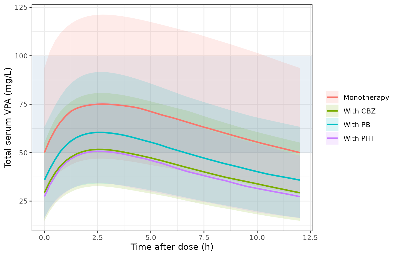
Simulated steady-state profiles by comedication arm (median and 5th-95th percentiles; 150 adults per arm; 500 mg gastro-resistant tablet every 12 h). The shaded band is the 50-100 mg/L therapeutic range.
obs <- sim |>
  filter(!is.na(Cc)) |>
  select(id, arm, time, Cc)
dose_df <- events |>
  filter(evid == 1) |>
  select(id, arm, time, amt)
nca_res <- PKNCA::pk.nca(PKNCA::PKNCAdata(
  PKNCA::PKNCAconc(obs, Cc ~ time | arm + id, concu = "mg/L", timeu = "h"),
  PKNCA::PKNCAdose(dose_df, amt ~ time | arm + id, doseu = "mg"),
  intervals = data.frame(start = 0, end = tau, cmax = TRUE, tmax = TRUE,
                         cmin = TRUE, cav = TRUE, auclast = TRUE)
))

as.data.frame(nca_res$result) |>
  group_by(arm, PPTESTCD) |>
  summarise(median = median(PPORRES, na.rm = TRUE), .groups = "drop") |>
  mutate(Parameter = nlmixr2lib::ncaParamLabel(PPTESTCD)) |>
  select(arm, Parameter, median) |>
  tidyr::pivot_wider(names_from = Parameter, values_from = median) |>
  rename("Arm" = arm) |>
knitr::kable(digits = 2, caption = "Median steady-state NCA over one 12 h interval by arm.")| Arm | AUClast | Cavg | Cmax | Cmin | Tmax |
|---|---|---|---|---|---|
| Monotherapy | 779.21 | 64.93 | 75.04 | 50.03 | 2.75 |
| With CBZ | 502.57 | 41.88 | 51.69 | 29.32 | 2.50 |
| With PB | 589.87 | 49.16 | 60.46 | 35.84 | 2.75 |
| With PHT | 481.05 | 40.09 | 50.68 | 27.32 | 2.50 |
At steady state Cav = Dose / (CL * tau) for every
subject. PKNCA’s cav must match the closed form computed
from each subject’s own clearance. Both sides use the same drawn
parameters, so the only difference is trapezoidal error on the 15-minute
grid.
cav_chk <- as.data.frame(nca_res$result) |>
  filter(PPTESTCD == "cav") |>
  select(id, cav = PPORRES) |>
  inner_join(sim |> distinct(id, cl), by = "id") |>
  mutate(cav_closed = 500 / (cl * tau), pct = 100 * (cav - cav_closed) / cav_closed)
stopifnot(all(abs(cav_chk$pct) < 1))
summary(cav_chk$pct)
#>      Min.   1st Qu.    Median      Mean   3rd Qu.      Max.
#> -0.058542 -0.032824 -0.026739 -0.027640 -0.021186 -0.009198
The paper publishes no NCA table, because its data are trough-only TDM samples. The Figure 2 comparison above is the published-exposure comparison.
Assumptions and deviations
- Carbamazepine coefficient. 0.521 (Equation (1) factor 1.521, confirmed by the Discussion) is used instead of Table 2’s 0.512, which reads as a transposed digit.
- Residual error. Table 2’s development-dataset RUV of 57.7% is inconsistent with its own bootstrap interval and with the Table 3 prediction errors. The bootstrap median of 28.1% is used (see above).
-
Variance scale. Table 2 reports the IIV and RUV as
CV%. They are converted with the log-normal identities
omega^2 = log(CV^2 + 1)andsd = sqrt(log(CV^2 + 1)). The alternativeomega = CVreading differs by 3.5% in variance at 26.8%. - No IIV on V/F. The control stream carries a V/F random effect with variance fixed at 0. It is omitted from the model file, which is equivalent and avoids a singular OMEGA.
-
Unknown formulation. In the source data a record
with unknown formulation (
FFS = 0) was given the gastro-resistant tablet Ka of 0.78 1/h, so it maps toFORM_TABLET = 1. Methods 2.3 describes imputing oral solution below 12 years and gastro-resistant tablet from 12 years. - Virtual cohort. Adults only, with age uniform on 19-89 years and weight log-normal around 70 kg (CV 20%, truncated to 40-125 kg). The paper does not publish per-age-group covariate distributions. Paediatric exposure is covered by the Figure 2 typical-patient replication.
-
Screened but not retained. Sex and lamotrigine were
significant in the forward step but changed CL/F by less than 10% and
were dropped. No coefficients are reported. They are listed in
covariatesDataExcluded.
Errata and internal inconsistencies in the source
- Table 2 carbamazepine coefficient reads 0.512. Equation (1) and the Discussion both correspond to 0.521.
- Table 2 RUV reads 57.7% (merged dataset 56.0%), far outside its own bootstrap 95% CI of 25.8-30.4%.
- Figure 2, 6-year / 21-kg panel sits below Equations (1) and (2) (peaks about 15% and troughs about 26% lower), while the other three panels reproduce them to within about 1% on peaks.
- Discussion typical clearances. The Discussion lists monotherapy CL/F of 0.010, 0.103, 0.538 and 1.484 L/h for typical patients of 1, 6, 15 and 35 years (9.4, 22.9, 53.3 and 73.5 kg). Equation (1) gives the values below. The ratios between comedication and monotherapy in those passages match Equation (1), but the absolute values do not. Figure 2, which the paper states was simulated with the final model, agrees with Equation (1).
| Age (y) | Weight (kg) | Discussion CL/F (L/h) | Equation (1) CL/F (L/h) |
|---|---|---|---|
| 1 | 9.4 | 0.010 | 0.149 |
| 6 | 22.9 | 0.103 | 0.283 |
| 15 | 53.3 | 0.538 | 0.527 |
| 35 | 73.5 | 1.484 | 0.661 |
- Patient count. The Abstract says the model was developed on “1751 samples from 776 patients”. Table 1, Supplementary Table S1 and Methods 2.1 all give 836 development patients; 776 is the number of external-evaluation samples.