Enoxaparin (Berges 2007)
Source:vignettes/articles/Berges_2007_enoxaparin.Rmd
Berges_2007_enoxaparin.RmdModel and source
- Citation: Berges A, Laporte S, Epinat M, Zufferey P, Alamartine E, Tranchand B, Decousus H, Mismetti P. Anti-factor Xa activity of enoxaparin administered at prophylactic dosage to patients over 75 years old. Br J Clin Pharmacol. 2007;64(4):428-438.
- Article: https://doi.org/10.1111/j.1365-2125.2007.02920.x
The Berges 2007 PROPHRE.75 model is a two-compartment first-order-absorption population PK model that describes anti-factor Xa (anti-Xa) activity as a surrogate for enoxaparin concentration after once-daily prophylactic subcutaneous injections of 4000 IU in elderly patients (>75 years). Body weight enters as a power-form covariate on apparent clearance and central volume, and creatinine clearance estimated by the simplified Modification of Diet in Renal Disease (MDRD) formula enters as a power-form covariate on apparent clearance.
Population
The PROPHRE.75 study (Berges 2007 Table 1) enrolled 189 elderly inpatients treated with subcutaneous enoxaparin 4000 IU once daily for VTE prophylaxis in medical and surgical contexts:
- Age: mean 82 +/- 5 years (range 75-95, median 81); 50% were over 81 years.
- Sex: 62% women.
- Weight: mean 66 +/- 14 kg (range 38-108); 22% under 55 kg; 8% obese (BMI > 30 kg/m^2).
- Renal function (median, range): Cockcroft-Gault CrCl 52 mL/min (24-93); simplified-MDRD CrCl 69 mL/min (27-127). Half had moderate or severe renal failure by Cockcroft-Gault (CrCl < 50 mL/min); only 18% by simplified MDRD.
- Indications: 63% immobility from acute medical disease, 15% orthopaedic surgery, 22% stroke.
- Common comorbidities: hypertension 57%, diabetes 24%, cancer 19%; 36% concomitant antiplatelet agents.
The mean duration of treatment was 7 days. A total of 451 anti-Xa activity samples were analysed (mean 2.4 per patient – very sparse).
The same information is available programmatically via
readModelDb("Berges_2007_enoxaparin") (e.g. inspect the
function body for the population metadata).
Source trace
The per-parameter origin is recorded as an in-file comment next to
each ini() entry in
inst/modeldb/specificDrugs/Berges_2007_enoxaparin.R. The
table below collects them in one place.
| Equation / parameter | Value | Source location |
|---|---|---|
lka (Ka) |
log(0.63 1/h) | Berges 2007 Table 3, KA row |
lcl (CL/F at WT=65, CRCL=69) |
log(0.70 L/h) | Berges 2007 Table 3, theta1 row |
lvc (V2/F at WT=65) |
log(6.43 L) | Berges 2007 Table 3, theta2 row |
lq (Q/F) |
log(0.34 L/h) | Berges 2007 Table 3, Q row |
lvp (V3/F) |
log(8.18 L) | Berges 2007 Table 3, V3 row |
e_wt_cl |
0.78 | Berges 2007 Table 3, theta6 row; Discussion confirms agreement with allometric 0.75 |
e_crcl_cl |
0.25 | Berges 2007 Table 3, theta7 row |
e_wt_vc |
1.25 | Berges 2007 Table 3, theta8 row; Discussion confirms agreement with allometric 1.0 |
etalcl (omega^2) |
0.0654 | Berges 2007 Table 3, CL IIV 26% CV converted via omega^2 = log(CV^2 + 1) |
etalvc (omega^2) |
0.0223 | Berges 2007 Table 3, V2 IIV 15% CV converted via omega^2 = log(CV^2 + 1) |
etalvp (omega^2) |
0.6229 | Berges 2007 Table 3, V3 IIV 93% CV converted via omega^2 = log(CV^2 + 1) |
| KA, Q IIV | 0 (fixed) | Berges 2007 Table 3, “0 FIXED” entries |
propSd |
0.30 | Berges 2007 Table 3, residual variability sigma row |
| Structural model | 2-compartment, first-order SC absorption | Berges 2007 Results > Model building |
| Covariate selection | weight + simplified-MDRD CrCl on CL, weight on V2 | Berges 2007 Table 2 (forward + backward selection, p < 0.01 backward); gender was dropped at backward elimination |
Virtual cohort
The PROPHRE.75 study did not release individual-level data; the simulations below use a virtual cohort whose demographics (weight, simplified-MDRD CrCl) were sampled to approximate Berges 2007 Table 1.
set.seed(2007)
n_subj <- 189L

# Weight: paper reports mean 66 +/- 14 kg, range 38-108. A truncated log-normal
# with the right mean and SD that respects the lower bound (38 kg) gives a
# defensible match without a published density. Resample any draw that falls
# outside the [38, 108] envelope (rejection sampling).
draw_truncated <- function(n, mean, sd, lower, upper, log_normal = FALSE) {
  out <- numeric(0)
  while (length(out) < n) {
    if (log_normal) {
      cv <- sd / mean
      sdlog <- sqrt(log(cv^2 + 1))
      meanlog <- log(mean) - sdlog^2 / 2
      draw <- rlnorm(n, meanlog = meanlog, sdlog = sdlog)
    } else {
      draw <- rnorm(n, mean = mean, sd = sd)
    }
    draw <- draw[draw >= lower & draw <= upper]
    out <- c(out, draw)
  }
  out[seq_len(n)]
}

cohort <- tibble(
  id   = seq_len(n_subj),
  WT   = draw_truncated(n_subj, mean = 66, sd = 14, lower = 38, upper = 108, log_normal = TRUE),
  CRCL = draw_truncated(n_subj, mean = 69, sd = 20, lower = 27, upper = 127)
)

summary(cohort[, c("WT", "CRCL")])
#>        WT              CRCL
#>  Min.   : 39.54   Min.   : 27.18
#>  1st Qu.: 57.66   1st Qu.: 56.71
#>  Median : 65.14   Median : 69.18
#>  Mean   : 66.20   Mean   : 69.57
#>  3rd Qu.: 73.95   3rd Qu.: 82.53
#>  Max.   :103.69   Max.   :115.73

# Build the event table for a 7-day prophylactic regimen (paper-reported mean
# treatment duration). Doses at 0, 24, 48, ... 144 h; observations every 0.5 h
# up to 168 h (one day after the last dose, so the simulation covers the full
# steady-state cycle).
dose_times <- seq(0, 144, by = 24)
obs_times  <- seq(0, 168, by = 0.5)

make_subject <- function(id, WT, CRCL) {
  doses <- tibble(
    id = id, time = dose_times, amt = 4000, cmt = "depot",
    evid = 1L, WT = WT, CRCL = CRCL
  )
  obs <- tibble(
    id = id, time = obs_times, amt = NA_real_, cmt = NA_character_,
    evid = 0L, WT = WT, CRCL = CRCL
  )
  bind_rows(doses, obs) |> arrange(time)
}

events <- lapply(
  seq_len(nrow(cohort)),
  function(i) make_subject(cohort$id[i], cohort$WT[i], cohort$CRCL[i])
) |> bind_rows()
stopifnot(!anyDuplicated(unique(events[, c("id", "time", "evid")])))
Simulation
mod <- readModelDb("Berges_2007_enoxaparin")
sim <- rxode2::rxSolve(mod, events = events, keep = c("WT", "CRCL"))
#> ℹ parameter labels from comments will be replaced by 'label()'
sim <- as.data.frame(sim)
Typical-value (zero random-effects) profile at the reference patient
(WT = 65, CRCL = 69):
mod_typical <- mod |> rxode2::zeroRe()
#> ℹ parameter labels from comments will be replaced by 'label()'
ev_typ <- tibble(
  id = 1L,
  time = c(dose_times, obs_times),
  amt  = c(rep(4000, length(dose_times)), rep(NA_real_, length(obs_times))),
  cmt  = c(rep("depot", length(dose_times)), rep(NA_character_, length(obs_times))),
  evid = c(rep(1L, length(dose_times)), rep(0L, length(obs_times))),
  WT   = 65,
  CRCL = 69
) |> arrange(time)
sim_typ <- as.data.frame(rxode2::rxSolve(mod_typical, events = ev_typ))
#> ℹ omega/sigma items treated as zero: 'etalcl', 'etalvc', 'etalvp'
Replicate published figures
# Replicates Figure 3 of Berges 2007: individual predictions vs. observations
# for four representative patients. The paper's plot showed observation + the
# individual-Bayesian fit; here we show a few simulated trajectories with
# different (WT, CRCL) draws from the virtual cohort to illustrate the typical
# concentration-time profile across the demographic range.
example_ids <- c(1L, 50L, 100L, 150L)
ex_sim <- sim |> filter(id %in% example_ids)
ggplot(ex_sim, aes(time, Cc, group = id)) +
  geom_line() +
  facet_wrap(~ id, labeller = function(x) {
    df <- cohort |> filter(id %in% example_ids)
    list(id = sprintf("ID %d (WT %.0f kg, CRCL %.0f mL/min)",
                     df$id, df$WT, df$CRCL))
  }) +
  labs(x = "Time (h)", y = "Anti-Xa activity (IU/mL)",
       title = "Simulated individual profiles",
       caption = "Replicates the form of Berges 2007 Figure 3 (individual predictions).")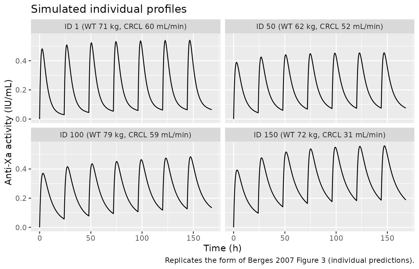
# Replicates Berges 2007 Results > Bayesian predictions: distribution of
# individual peak anti-Xa activities between 3-5 h after subcutaneous
# injection. Paper reports range 0.10-1.20 IU/mL, median 0.44; 29% > 0.5, 10% > 0.8,
# 4% > 1.0.
peak_window <- sim |>
  group_by(id) |>
  filter(time >= 144 + 3, time <= 144 + 5) |>   # peak window after the final dose
  summarise(peak = max(Cc, na.rm = TRUE), .groups = "drop")

paper_thresholds <- tibble(
  threshold_IU_mL = c(0.5, 0.8, 1.0),
  paper_pct       = c(29, 10, 4)
)
sim_pct <- paper_thresholds |>
  mutate(sim_pct = sapply(threshold_IU_mL,
                          function(th) 100 * mean(peak_window$peak > th)))
print(sim_pct)
#> # A tibble: 3 × 3
#>   threshold_IU_mL paper_pct sim_pct
#>             <dbl>     <dbl>   <dbl>
#> 1             0.5        29   40.7
#> 2             0.8        10    1.59
#> 3             1           4    0

ggplot(peak_window, aes(peak)) +
  geom_histogram(bins = 30, fill = "grey70", colour = "grey30") +
  geom_vline(xintercept = c(0.5, 0.8, 1.0), colour = "tomato", linetype = "dashed") +
  labs(x = "Peak anti-Xa activity, 3-5 h post-dose (IU/mL)",
       y = "Number of simulated subjects",
       title = "Distribution of individual peak anti-Xa activity (steady state)",
       caption = paste0("Replicates Berges 2007 Bayesian-predictions paragraph. ",
                        "Paper reports median 0.44, range 0.10-1.20 IU/mL; ",
                        "29% > 0.5, 10% > 0.8, 4% > 1.0."))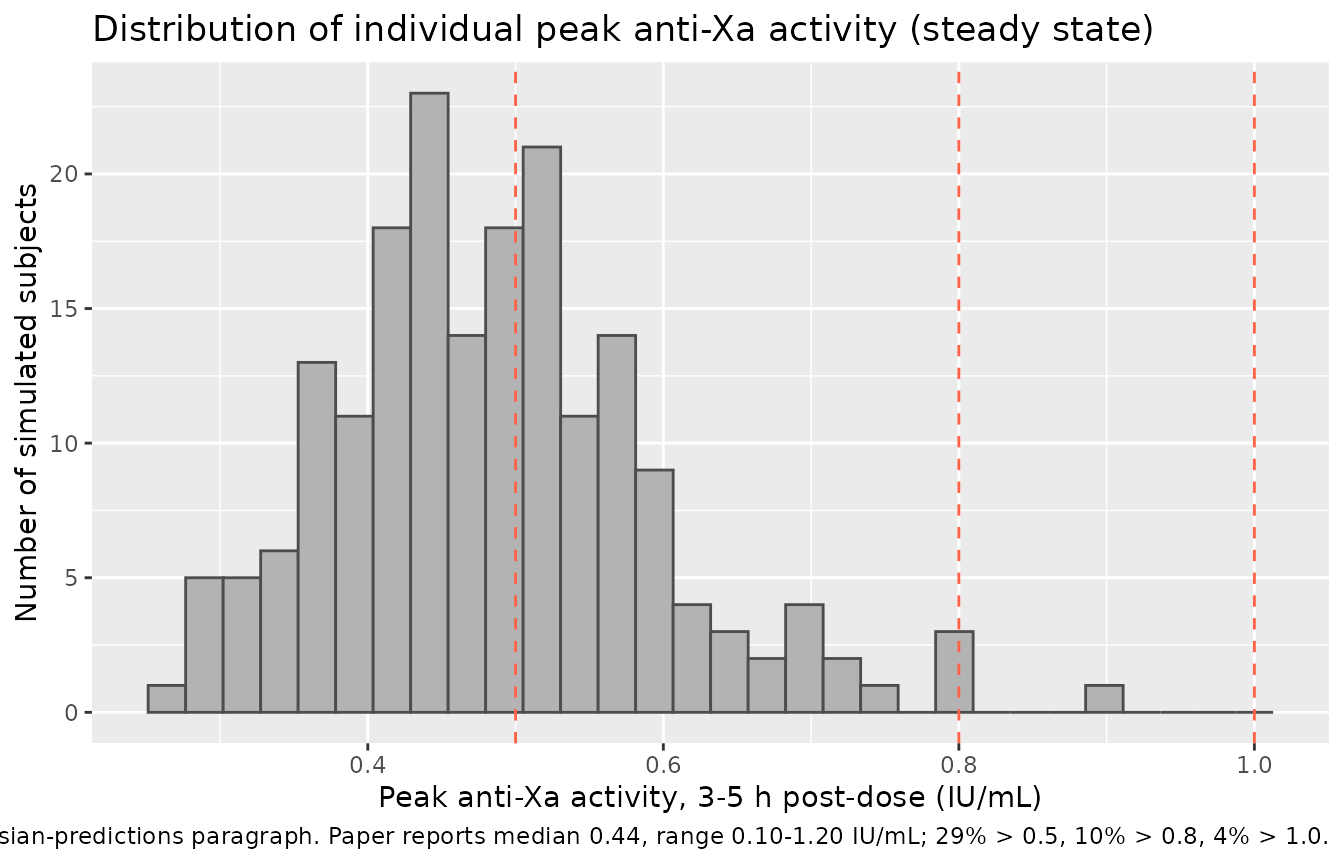
PKNCA validation
PKNCA is run on the per-cycle steady-state interval (the final 24-hour dosing interval, 144-168 h) so the reported NCA reflects steady-state prophylactic dosing.
sim_nca <- sim |>
  dplyr::filter(!is.na(Cc)) |>
  dplyr::select(id, time, Cc, WT, CRCL) |>
  dplyr::mutate(treatment = "Enoxaparin 4000 IU SC QD")

# Guarantee a time = 0 row per subject (extravascular pre-dose Cc = 0).
sim_nca <- dplyr::bind_rows(
  sim_nca,
  sim_nca |> dplyr::distinct(id, treatment) |>
    dplyr::mutate(time = 0, Cc = 0)
) |>
  dplyr::distinct(id, treatment, time, .keep_all = TRUE) |>
  dplyr::arrange(id, treatment, time)

conc_obj <- PKNCA::PKNCAconc(
  sim_nca, Cc ~ time | treatment + id,
  concu = "IU/mL", timeu = "h"
)

dose_df <- events |>
  dplyr::filter(evid == 1) |>
  dplyr::select(id, time, amt) |>
  dplyr::mutate(treatment = "Enoxaparin 4000 IU SC QD")

dose_obj <- PKNCA::PKNCAdose(
  dose_df, amt ~ time | treatment + id,
  doseu = "IU"
)

# Steady-state interval: the last full dosing cycle (144-168 h).
intervals <- data.frame(
  start    = 144,
  end      = 168,
  cmax     = TRUE,
  tmax     = TRUE,
  cmin     = TRUE,
  auclast  = TRUE,
  cav      = TRUE
)

nca_res <- PKNCA::pk.nca(PKNCA::PKNCAdata(conc_obj, dose_obj, intervals = intervals))
Comparison against published anti-Xa peak distribution
Berges 2007 does not tabulate Cmax / Tmax / AUC as a formal NCA, but the Bayesian-predictions paragraph reports the median peak anti-Xa activity in the 3-5 h post-dose window and the fraction of subjects above three clinically interesting thresholds (0.5, 0.8, 1.0 IU/mL).
sim_peak_summary <- tibble(
  treatment    = "Enoxaparin 4000 IU SC QD",
  median_peak  = median(peak_window$peak),
  min_peak     = min(peak_window$peak),
  max_peak     = max(peak_window$peak),
  pct_gt_0_5   = round(100 * mean(peak_window$peak > 0.5), 1),
  pct_gt_0_8   = round(100 * mean(peak_window$peak > 0.8), 1),
  pct_gt_1_0   = round(100 * mean(peak_window$peak > 1.0), 1)
)
sim_peak_summary
#> # A tibble: 1 × 7
#>   treatment       median_peak min_peak max_peak pct_gt_0_5 pct_gt_0_8 pct_gt_1_0
#>   <chr>                 <dbl>    <dbl>    <dbl>      <dbl>      <dbl>      <dbl>
#> 1 Enoxaparin 400…       0.478    0.264    0.892       40.7        1.6          0

published_peak <- tibble::tibble(
  treatment    = "Enoxaparin 4000 IU SC QD",
  median_peak  = 0.44,
  min_peak     = 0.10,
  max_peak     = 1.20,
  pct_gt_0_5   = 29,
  pct_gt_0_8   = 10,
  pct_gt_1_0   = 4
)

cmp <- bind_rows(
  sim_peak_summary |> mutate(source = "Simulated"),
  published_peak  |> mutate(source = "Berges 2007 (Bayesian predictions)")
) |> relocate(source)

knitr::kable(
  cmp,
  caption = "Steady-state peak anti-Xa (3-5 h post final dose): simulated virtual cohort vs Berges 2007 Bayesian predictions.",
  digits  = 2
)| source | treatment | median_peak | min_peak | max_peak | pct_gt_0_5 | pct_gt_0_8 | pct_gt_1_0 |
|---|---|---|---|---|---|---|---|
| Simulated | Enoxaparin 4000 IU SC QD | 0.48 | 0.26 | 0.89 | 40.7 | 1.6 | 0 |
| Berges 2007 (Bayesian predictions) | Enoxaparin 4000 IU SC QD | 0.44 | 0.10 | 1.20 | 29.0 | 10.0 | 4 |
PKNCA steady-state per-subject Cmax / Tmax / AUC0-tau summary (no published counterpart):
nca_tbl <- as.data.frame(nca_res$result)
nca_summary <- nca_tbl |>
  dplyr::group_by(PPTESTCD) |>
  dplyr::summarise(
    median = signif(median(PPORRES, na.rm = TRUE), 3),
    q05    = signif(quantile(PPORRES, 0.05, na.rm = TRUE), 3),
    q95    = signif(quantile(PPORRES, 0.95, na.rm = TRUE), 3),
    .groups = "drop"
  )
knitr::kable(
  nca_summary,
  caption = "Steady-state NCA summary (144-168 h cycle, virtual PROPHRE.75-like cohort)."
)| PPTESTCD | median | q05 | q95 |
|---|---|---|---|
| auclast | 5.8400 | 3.5500 | 8.800 |
| cav | 0.2430 | 0.1480 | 0.367 |
| cmax | 0.4780 | 0.3210 | 0.699 |
| cmin | 0.0915 | 0.0387 | 0.187 |
| tmax | 3.0000 | 2.5000 | 3.500 |
Assumptions and deviations
-
Block matrix correlation between CL and V2 is set to
zero. Berges 2007 Results > Model building states that “A
block matrix was added to take into account the correlation between CL
and V2,” but Table 3 reports only the diagonal CV%s; the off-diagonal
covariance value is not published. The model encodes diagonal etas for
etalclandetalvc(no block); the paper-reported CL and V2 %CVs are preserved on the diagonal. A simulator who has an internal estimate of the correlation can re-introduce a block viaini(etalcl + etalvc ~ c(var_cl, cov, var_vc)). - Virtual-cohort covariate sampling. The PROPHRE.75 study did not release individual-level data; weight is drawn from a truncated log-normal matched to Berges 2007 Table 1 (mean 66 kg, SD 14 kg, truncated to [38, 108]), and simplified-MDRD CrCl from a truncated normal (mean 69 mL/min, SD 20, truncated to [27, 127]). Sex, indication category, and concomitant medications are not simulated because they were not retained in the final covariate model.
- Gender effect on CL is excluded. Berges 2007 Table 2 retained gender on CL through forward selection (p < 0.01) but dropped it at backward elimination (p < 0.02 did not meet the < 0.01 threshold). Table 3 final-parameter estimates do not include a gender effect; the model file faithfully omits it.
-
Anti-Xa activity vs enoxaparin concentration.
Heparin concentration cannot be measured directly; anti-Xa activity
(IU/mL) is the surrogate endpoint used throughout the paper and is what
the model predicts as
Cc. Apparent V2 = V2/F absorbs subcutaneous bioavailability; the model does not estimate F separately. - Below-LOQ handling. Berges 2007 excluded 56 of 451 anti-Xa activity samples below the assay LOQ (0.05 IU/mL) from estimation. The simulation emits continuous concentrations; no BLQ rule is applied at simulation time.