Linezolid continuous versus intermittent infusion (Hui 2024)
Source:vignettes/articles/Hui_2024_linezolid.Rmd
Hui_2024_linezolid.RmdModel and source
Citation: Hui LA, Bodolea C, Popa A, Vlase AM, Hiriscau EI, Vlase L (2024). Linezolid Pharmacokinetics in Critically Ill Patients: Continuous Versus Intermittent Infusion. Antibiotics (Basel) 13(10):961. doi:10.3390/antibiotics13100961
Description (intermittent arm): Two-compartment pharmacokinetic model with first-order elimination for intravenous linezolid given as an intermittent infusion (600 mg over 1-2 h every 12 h) to critically ill adults in an intensive care unit (Hui 2024, intermittent-infusion arm, n = 15). Hui 2024 fitted each patient individually in Phoenix WinNonlin, selected the two-compartment model over the one-compartment model by AIC, and reported only summary statistics (mean, SD, CV% and median) of the individual estimates per infusion arm (Table 2). This is therefore a typical-value model, not a population model: every parameter is fixed at the arm’s median individual estimate of CL, V1, V2 and the distribution clearance CLD2, and there is no between-subject variability or residual-error model (residual SD fixed at zero). Covariates were only screened by ANOVA on the individual estimates (Table 4) and none enters the model. The continuous-infusion arm of the same study is modellib(‘Hui_2024_linezolid_continuous’).
Description (continuous arm): Two-compartment pharmacokinetic model with first-order elimination for intravenous linezolid given as a continuous infusion (600 mg loading infusion over 1 h, then 1200 mg/day at 50 mg/h) to critically ill adults in an intensive care unit (Hui 2024, continuous-infusion arm, n = 14). Hui 2024 fitted each patient individually in Phoenix WinNonlin, selected the two-compartment model over the one-compartment model by AIC, and reported only summary statistics (mean, SD, CV% and median) of the individual estimates per infusion arm (Table 2). This is therefore a typical-value model, not a population model: every parameter is fixed at the arm’s median individual estimate of CL, V1, V2 and the distribution clearance CLD2, and there is no between-subject variability or residual-error model (residual SD fixed at zero). Covariates were only screened by ANOVA on the individual estimates (Table 4) and none enters the model. The intermittent-infusion arm of the same study is modellib(‘Hui_2024_linezolid_intermittent’).
Supplement (Table S1, a literature summary with no model parameters): https://www.mdpi.com/article/10.3390/antibiotics13100961/s1
Hui 2024 compares the same daily linezolid dose (1200 mg/day) given to critically ill adults either as a conventional intermittent infusion (II) or as a continuous infusion (CI) after a loading dose. Each patient’s serum concentrations were fitted individually with the standard one- and two-compartment models of Phoenix WinNonlin 6.3; the two-compartment model had the lower AIC and was retained (Methods 4.8). The paper then reports, per infusion arm, the mean, SD, CV% and median of the individual estimates (Table 2). There is no population (nonlinear mixed-effects) fit, so there is no typical-value estimate, no between-subject variance and no residual-error model in the source.
The library therefore carries one typical-value two-compartment model per arm, each fixed at that arm’s median individual CL, V1, V2 and distribution clearance CLD2:
-
Hui_2024_linezolid_intermittent– 15 patients, 600 mg over 1-2 h every 12 h. -
Hui_2024_linezolid_continuous– 14 patients, 600 mg over 1 h, then 50 mg/h.
The two files share one structure and differ only in their parameter values; the paper found no statistically significant effect of the infusion method on any individual parameter (Table 4, “Treatment” column, p >= 0.078).
Population
Twenty-nine of 55 screened patients were analysed: 14 in the CI arm (the first four months of the study, the ward’s standard practice) and 15 in the II arm (the following four months), at the intensive care unit of the University Clinical Municipal Hospital, Cluj-Napoca, Romania, between July 2022 and March 2023 (NCT05801484; Results 2.1, Methods 4.1-4.2). All were Caucasian; 7 were women. Age ranged 45-87 years; the II arm was older (median 75 vs 72 years, p = 0.043). Mean weight was 85.8 kg (II) and 77.7 kg (CI); mean SOFA 8.7 and 10.7; septic shock was present in 11/15 and 7/14 (Table 1). Renal function spanned augmented clearance (CrCl > 130 mL/min, 3 CI patients) to CrCl below 15 mL/min (3 patients), and 15 patients were Child-Pugh B; some received CVVHDF or intermittent haemodialysis. Serum was sampled before the first infusion, at 1, 2, 4, 8, 12, 16, 24, 36 and 48 h, and then daily until the end of treatment (2-13 days); 396 samples were assayed by LC-MS (LOQ 0.256 ug/mL).
The same information is available programmatically via the model’s
population metadata:
str(readModelDb("Hui_2024_linezolid_continuous")()$population[c("n_subjects", "age_median", "weight_mean", "sex_female_pct")])
#> List of 4
#>  $ n_subjects    : num 14
#>  $ age_median    : chr "72.0 years (IQR 61.0-80.0)"
#>  $ weight_mean   : chr "77.7 kg (SD 22.7)"
#>  $ sex_female_pct: num 14.3
Source trace
The per-parameter origin is recorded as an in-file comment next to
each ini() entry in
inst/modeldb/specificDrugs/Hui_2024_linezolid_intermittent.R
and Hui_2024_linezolid_continuous.R.
| Equation / parameter | II value | CI value | Source location |
|---|---|---|---|
lcl (CL, L/h) |
log(5.36) | log(5.66) | Table 2, CL median per group |
lvc (V1, L) |
log(40.99) | log(35.91) | Table 2, V1 median per group |
lvp (V2, L) |
log(24.01) | log(23.75) | Table 2, V2 median per group |
lq (CLD2, L/h) |
log(18.16) | log(10.01) | Table 2, CLD2 median per group |
addSd |
0 | 0 | not reported (individual WinNonlin fits) |
| Two-compartment structure, first-order elimination from central | n/a | n/a | Methods 4.8 (selected over one-compartment by AIC); parameter list in Table 2 footnote |
| II regimen: 600 mg over 1 or 2 h every 12 h | n/a | n/a | Methods 4.4 |
| CI regimen: 600 mg over 1 h, then 1200 mg/day at 50 mg/h | n/a | n/a | Methods 4.4 |
Simulation
The models carry no random effects, so each simulation is one typical patient per arm. The infusion is 1 h in both arms (the II protocol allowed 1 or 2 h); the continuous infusion is taken to start when the loading infusion ends.
t_end <- 168
obs_times <- sort(unique(c(seq(0, t_end, by = 0.25), 24, 48, 72)))

ev_ii <- rxode2::et(amt = 600, rate = 600, cmt = "central", ii = 12, addl = t_end / 12 - 1) |>
  rxode2::et(obs_times, cmt = "central") |>
  as.data.frame() |>
  dplyr::mutate(id = 1L, treatment = "II")

ev_ci <- rxode2::et(amt = 600, rate = 600, cmt = "central") |>
  rxode2::et(time = 1, amt = 50 * (t_end - 1), rate = 50, cmt = "central") |>
  rxode2::et(obs_times, cmt = "central") |>
  as.data.frame() |>
  dplyr::mutate(id = 2L, treatment = "CI")
mod_ii <- readModelDb("Hui_2024_linezolid_intermittent")
mod_ci <- readModelDb("Hui_2024_linezolid_continuous")

sim_ii <- rxode2::rxSolve(mod_ii, events = ev_ii, keep = "treatment")
sim_ci <- rxode2::rxSolve(mod_ci, events = ev_ci, keep = "treatment")

# A single-subject solve returns no `id` column; restore it from the arm.
sim <- dplyr::bind_rows(as.data.frame(sim_ii), as.data.frame(sim_ci)) |>
  dplyr::mutate(id = ifelse(treatment == "II", 1L, 2L), parameter_set = "Median (packaged)")
Table 2 also reports the mean of each individual
parameter. To show how much the choice of summary statistic matters for
this skewed, small cohort, the same regimens are simulated with the mean
parameter set substituted through params.
mean_ii <- c(lcl = log(7.88), lvc = log(47.46), lvp = log(26.50), lq = log(29.47))
mean_ci <- c(lcl = log(6.95), lvc = log(36.99), lvp = log(26.17), lq = log(15.43))

sim_mean <- dplyr::bind_rows(
  as.data.frame(rxode2::rxSolve(mod_ii, events = ev_ii, params = mean_ii, keep = "treatment")),
  as.data.frame(rxode2::rxSolve(mod_ci, events = ev_ci, params = mean_ci, keep = "treatment"))
) |>
  dplyr::mutate(parameter_set = "Mean (Table 2)")

# The substitution must actually take effect: the mean-set CL differs from
# the median-set CL by 30-50%, so the steady-state level must move.
stopifnot(
  abs(sim_mean$Cc[sim_mean$treatment == "CI" & sim_mean$time == t_end] -
    sim$Cc[sim$treatment == "CI" & sim$time == t_end]) > 1
)
sim_all <- dplyr::bind_rows(sim, sim_mean)
Structural checks
With no random effects, two closed-form identities must hold on the
numeric (ODE) solution. During the continuous infusion, the
concentration approaches R / CL; for the intermittent
regimen at steady state, the AUC over one 12-h dosing interval equals
Dose / CL.
css_ci_analytic <- 50 / exp(ui_ci$theta[["lcl"]])
css_ci_sim <- sim$Cc[sim$treatment == "CI" & sim$time == t_end]

ii_last <- sim |>
  dplyr::filter(treatment == "II", time >= t_end - 12, time <= t_end)
auc_tau_sim <- sum(diff(ii_last$time) * (head(ii_last$Cc, -1) + tail(ii_last$Cc, -1)) / 2)
auc_tau_analytic <- 600 / exp(ui_ii$theta[["lcl"]])

data.frame(
  check = c("CI concentration at 168 h vs 50 mg/h / CL", "II AUC(156-168 h) vs 600 mg / CL"),
  simulated = c(css_ci_sim, auc_tau_sim),
  analytic = c(css_ci_analytic, auc_tau_analytic)
) |>
  dplyr::mutate(pct_diff = 100 * (simulated / analytic - 1)) |>
knitr::kable(digits = 3)| check | simulated | analytic | pct_diff |
|---|---|---|---|
| CI concentration at 168 h vs 50 mg/h / CL | 8.834 | 8.834 | 0 |
| II AUC(156-168 h) vs 600 mg / CL | 111.940 | 111.940 | 0 |
stopifnot(
  # 168 h is about 20 terminal half-lives (8.1 h), so the approach to
  # steady state is complete to well under 0.1%.
  abs(css_ci_sim / css_ci_analytic - 1) < 1e-3,
  # Linear trapezoid on a 0.25-h grid over one steady-state interval;
  # measured about 2e-6 relative, so the bound keeps over 100-fold headroom.
  abs(auc_tau_sim / auc_tau_analytic - 1) < 1e-3
)
Replicate published figures
Figure 3 of Hui 2024 overlays the individual fitted profiles of every patient (II: panel a, CI: panel b). The typical profiles below sit inside the bands the paper describes: II profiles oscillate between roughly 0 and 25 ug/mL, and CI profiles settle between 3 and 15 ug/mL after the loading peak (Results 2.2).
sim_all |>
  dplyr::mutate(treatment = factor(treatment, c("II", "CI"),
    c("Intermittent infusion (600 mg q12h)", "Continuous infusion (600 mg load + 50 mg/h)"))) |>
  ggplot(aes(time, Cc, colour = parameter_set)) +
  geom_line() +
  facet_wrap(~treatment, ncol = 1) +
  labs(
    x = "Time (h)", y = "Linezolid serum concentration (ug/mL)", colour = "Parameter set",
    caption = "Typical-value analogue of Figure 3 of Hui 2024 (individual fitted profiles)."
  ) +
  theme_bw() +
  theme(legend.position = "bottom")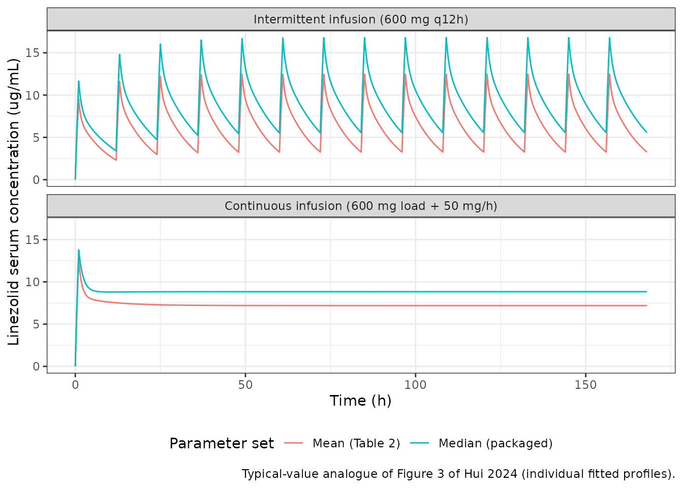
Figure 4 of Hui 2024 is the probability of target attainment across patients. It cannot be reproduced from a typical-value model, which has no between-patient distribution; the typical patient’s AUC24-48/MIC is listed below for reference against the 80 target.
auc_24_48 <- sim |>
  dplyr::filter(time >= 24, time <= 48) |>
  dplyr::group_by(treatment) |>
  dplyr::summarise(auc = sum(diff(time) * (head(Cc, -1) + tail(Cc, -1)) / 2), .groups = "drop")

tidyr::expand_grid(auc_24_48, mic = c(1, 2, 4)) |>
  dplyr::mutate(auc_mic = auc / mic, target_met = auc_mic >= 80) |>
  dplyr::rename("Arm" = treatment, "AUC24-48 (ug*h/mL)" = auc, "MIC (ug/mL)" = mic,
    "AUC24-48/MIC" = auc_mic, "AUC/MIC >= 80" = target_met) |>
knitr::kable(digits = 1, caption = "Typical patient, median parameter set.")| Arm | AUC24-48 (ug*h/mL) | MIC (ug/mL) | AUC24-48/MIC | AUC/MIC >= 80 |
|---|---|---|---|---|
| CI | 211.9 | 1 | 211.9 | TRUE |
| CI | 211.9 | 2 | 106.0 | TRUE |
| CI | 211.9 | 4 | 53.0 | FALSE |
| II | 214.9 | 1 | 214.9 | TRUE |
| II | 214.9 | 2 | 107.5 | TRUE |
| II | 214.9 | 4 | 53.7 | FALSE |
The typical patient reaches the target at MIC 1 and 2 ug/mL in both arms and misses it at 4 ug/mL. Table 3 reports attainment in 87%/100% (MIC 1), 60%/64% (MIC 2) and 27%/21% (MIC 4) of II/CI patients, so the typical patient sits where the population is split near MIC 2 and below the target at MIC 4, as the paper describes.
PKNCA validation
sim_nca <- sim |>
  dplyr::filter(!is.na(Cc)) |>
  dplyr::select(id, time, Cc, treatment)
sim_nca <- dplyr::bind_rows(
  sim_nca,
  sim_nca |> dplyr::distinct(id, treatment) |> dplyr::mutate(time = 0, Cc = 0)
) |>
  dplyr::distinct(id, treatment, time, .keep_all = TRUE) |>
  dplyr::arrange(id, treatment, time)

dose_df <- dplyr::bind_rows(ev_ii, ev_ci) |>
  dplyr::filter(!is.na(amt), amt > 0) |>
  dplyr::select(id, time, amt, treatment)

conc_obj <- PKNCA::PKNCAconc(sim_nca, Cc ~ time | treatment + id)
dose_obj <- PKNCA::PKNCAdose(dose_df, amt ~ time | treatment + id)

intervals <- data.frame(
  start = c(0, 24, 48),
  end = c(24, 48, 72),
  cmax = c(TRUE, FALSE, FALSE),
  auclast = TRUE
)
nca_res <- PKNCA::pk.nca(PKNCA::PKNCAdata(conc_obj, dose_obj, intervals = intervals))
Comparison against published values
Table 3 reports the AUC over 24-48 h and 48-72 h, and Table 2 the Cmax, as summaries of the individual fitted profiles. The AUC rows have only a mean (Table 3); Cmax is compared with its median (Table 2), which is the matching statistic for a median-parameter typical patient.
Table 2’s “AUC0-24” is not compared. Its II median, 111.91 ugh/mL, equals 600 mg divided by the II median CL (600 / 5.36 = 111.94), and Table 4 assigns AUC and CL identical p-values for every covariate – the column is the Phoenix single-dose secondary parameter Dose/CL, a transform of CL rather than an exposure over the first day (see Assumptions and deviations*).
sim_long <- as.data.frame(nca_res$result) |>
  dplyr::mutate(interval = paste0(start, "-", end, " h")) |>
  dplyr::select(treatment, interval, PPTESTCD, PPORRES)

published <- tibble::tribble(
  ~treatment, ~interval, ~cmax, ~auclast,
  "II", "0-24 h", 11.35, NA,
  "II", "24-48 h", NA, 224.87,
  "II", "48-72 h", NA, 236.40,
  "CI", "0-24 h", 13.49, NA,
  "CI", "24-48 h", NA, 205.23,
  "CI", "48-72 h", NA, 222.04
)

# Compare only the (arm, interval, parameter) cells the paper reports.
published_cells <- published |>
  tidyr::pivot_longer(c(cmax, auclast), names_to = "PPTESTCD", values_to = "ref") |>
  dplyr::filter(!is.na(ref)) |>
  dplyr::select(treatment, interval, PPTESTCD)
stopifnot(nrow(published_cells) == 6)

cmp <- nlmixr2lib::ncaComparisonTable(
  simulated = dplyr::semi_join(sim_long, published_cells, by = c("treatment", "interval", "PPTESTCD")),
  reference = published,
  by = c("treatment", "interval"),
  units = c(cmax = "ug/mL", auclast = "ug*h/mL"),
  tolerance_pct = 20
)
knitr::kable(cmp, caption = "Simulated typical patient vs. Hui 2024 Tables 2-3. * differs from the reference by more than 20%.")| NCA parameter | treatment | interval | Reference | Simulated | % diff |
|---|---|---|---|---|---|
| Cmax (ug/mL) | II | 0-24 h | 11.4 | 14.8 | +30.5%* |
| Cmax (ug/mL) | CI | 0-24 h | 13.5 | 13.8 | +2.1% |
| AUClast (ug*h/mL) | II | 24-48 h | 225 | 215 | -4.4% |
| AUClast (ug*h/mL) | II | 48-72 h | 236 | 223 | -5.9% |
| AUClast (ug*h/mL) | CI | 24-48 h | 205 | 212 | +3.3% |
| AUClast (ug*h/mL) | CI | 48-72 h | 222 | 212 | -4.5% |
sim_auc <- sim_long |>
  dplyr::filter(PPTESTCD == "auclast", interval != "0-24 h") |>
  dplyr::left_join(published |> dplyr::select(treatment, interval, auclast), by = c("treatment", "interval"))
# The typical patient must land within 10% of the published mean AUC (measured
# 3-6%; the model has no random effects, so this does not vary by machine): a
# mis-transcribed clearance or dose moves every interval by far more. The
# mean of individual AUCs exceeds the AUC of the median patient (Jensen's
# inequality on Dose/CL), so the comparison is expected to sit slightly low.
stopifnot(nrow(sim_auc) == 4, all(abs(sim_auc$PPORRES / sim_auc$auclast - 1) < 0.10))
The typical-patient AUCs over 24-48 h and 48-72 h fall within 6% of the published means in both arms (three of the four are lower). Some shortfall is expected: the mean of individual AUCs is pulled up by the patients with the lowest clearance (Discussion: a CI patient with CrCl below 15 mL/min had an AUC24-48 of 261 ug*h/mL and a half-life of 28 h), while a typical patient carries the median clearance.
The CI Cmax, the end of the loading infusion, matches the Table 2 median to 2%. The II Cmax is 30% above it (flagged). Part of the gap is the infusion length: the protocol allowed 1- or 2-h infusions, and a 2-h infusion lowers the typical first-day peak from 14.8 to 13.1 ug/mL (+16% against the median). The remainder is not resolvable from the paper, which does not say over which interval, or from which dose, Cmax was read; the parameters were not adjusted.
Assumptions and deviations
-
A typical-value model built from summary
statistics. Hui 2024 fitted every patient separately and
published the distribution of the individual estimates, not a population
model. The SDs in Table 2 mix true between-patient variability with each
patient’s estimation error, so they were not reinterpreted as
between-subject variances; the models carry no
etaterms and the residual SD is fixed at zero. This follows the convention used for other individual-fit papers in the library (for exampleMo_2024_shikimicAcid_pig_iv). - Median rather than mean. The individual estimates are strongly right-skewed (CV 46-118% for CL, V1, V2 and CLD2; the means of CL and CLD2 are 1.2-1.6 times the medians). The maintainers took the median as the typical value because, unlike the mean, it is unchanged by the monotone transforms that link a parameter to its rate constant or half-life, and it corresponds to the typical value of a log-normal population model. For the II arm the four medians are also mutually consistent: they give alpha = 1.25 /h, beta = 0.079 /h and half-lives of 0.55 h and 8.8 h, against the tabulated medians 1.21 /h, 0.07 /h, 0.57 h and 9.25 h. For the CI arm the agreement is looser (alpha 0.77 vs 0.56 /h; beta half-life 8.1 vs 6.2 h), because a continuous infusion carries little information on the distribution phase. The mean set is shown alongside above for comparison.
- Medians of individual parameters are not one patient. The medians of CL, V1, V2 and CLD2 come from different patients, so the derived rate constants (II: K10 0.131, K12 0.443, K21 0.756 /h; CI: 0.158, 0.279, 0.421 /h) do not equal the tabulated medians of K10, K12 and K21 (II: 0.10, 0.29, 0.44 /h; CI: 0.23, 0.16, 0.22 /h). The clearance parameterisation was packaged because it is the library’s convention; which parameterisation Phoenix estimated directly is not stated.
- Table 2 “AUC0-24” is Dose/CL. Its II median (111.91 ug*h/mL) equals 600 mg / 5.36 L/h = 111.94, and with 15 patients the median is a single patient’s value, so the identity is exact to rounding. Table 4 also gives AUC and CL identical p-values for all eight covariates (as it does for Alpha and Alpha_HL, and for Beta and Beta_HL, which are exact transforms of each other). The column is therefore the single-dose AUC from zero to infinity of a 600 mg dose, not the exposure over the first 24 h, and is not used as a validation target. The CI median (109.29) is consistent with the same reading (with 14 patients the median averages two values, so it need not equal 600 / 5.66 exactly).
- Cmax. The paper does not state over which interval Cmax was read. The typical II patient’s first-day peak (1-h infusion) is compared with the Table 2 median and is 30% higher; with a 2-h infusion it is 16% higher, and the steady-state peak is higher still (16.8 ug/mL). The paper reports a lower mean Cmax for II (10.91) than for CI (13.58) and does not explain it. For the CI arm, Cmax is the end of the loading infusion.
- Infusion timing. The II protocol allowed 1- or 2-h infusions; 1 h is simulated. The CI is assumed to start immediately after the 1-h loading infusion; the paper does not state the gap.
-
Covariates. Table 4 tests sex, age, hepatic and
renal function, albumin, renal replacement therapy and BMI against each
individual parameter by ANOVA and reports p-values only. Sex reached
significance for CLD2, K12, V2 and Cmax, but no effect size is reported,
so no covariate enters either model; the screen is documented in each
model’s
covariatesDataExcluded. - No erratum or correction notice was found for Hui 2024 (Europe PMC, checked 2026-10-31).