Recombinant vs plasma-derived von Willebrand factor (Bauer 2023) • nlmixr2lib

Model and source

Bauer 2023 developed two population PK/PD models, one per product, and used them for an in-silico comparison in von Willebrand disease (VWD) type 3. This paper therefore contributes two model files, both documented here.

Article: https://doi.org/10.2147/JBM.S395845
Supplement: https://www.dovepress.com/get_supplementary_file.php?f=395845.docx

mod_rvwf <- readModelDb("Bauer_2023_vonicogAlfa")
mod_pd   <- readModelDb("Bauer_2023_vwfFviii_humateP")

rxode2::rxode(mod_rvwf)$reference
#> ℹ parameter labels from comments will be replaced by 'label()'
#> [1] "Bauer A, Friberg-Hietala S, Smania G, Wolfsegger M. Pharmacokinetic-pharmacodynamic comparison of recombinant and plasma-derived von Willebrand factor in patients with von Willebrand disease type 3. J Blood Med. 2023;14:399-411. doi:10.2147/JBM.S395845."

Recombinant von Willebrand factor (rVWF, vonicog alfa):

rxode2::rxode(mod_rvwf)$description
#> ℹ parameter labels from comments will be replaced by 'label()'
#> [1] "Two-compartment population PK model for von Willebrand factor:ristocetin cofactor activity (VWF:RCo) after intravenous recombinant von Willebrand factor (rVWF, vonicog alfa) coupled to an indirect-response PK/PD model for endogenous factor VIII activity (FVIII:C), from Bauer 2023. VWF:RCo disposition is linear two-compartment with first-order elimination from the central compartment plus an additive endogenous background activity E_VWF, fixed at half the assay LLOQ (0.5 IU/dL) for von Willebrand disease (VWD) type 3. CL and Q are allometrically scaled by body weight with a fixed exponent of 0.75, Vc and Vp with a fixed exponent of 1, both referenced to 75 kg; Vc additionally decreases with hematocrit as (HCT/40)^-0.334. FVIII:C is a turnover pool with zero-order production kin = FVIII0 * kout and first-order removal kout (15.9 1/h) that VWF:RCo inhibits through an Imax function, 1 - Imax * VWF:RCo / (IC50 + VWF:RCo), so that rising VWF:RCo protects FVIII from clearance; FVIII0 is the theoretical baseline FVIII:C at VWF:RCo = 0 IU/dL and scales with hematocrit as (HCT/39)^-0.571. Fitted to 1664 VWF:RCo samples from 79 patients across four studies (VWD types 1, 2, 3 and severe hemophilia A) and 686 FVIII:C samples from the 41 patients of the two phase 3 VWD studies."

Plasma-derived von Willebrand factor / factor VIII concentrate (pdVWF/FVIII; Humate-P, VWF:RCo/FVIII:C 2.4:1):

rxode2::rxode(mod_pd)$description
#> ℹ parameter labels from comments will be replaced by 'label()'
#> [1] "Two-compartment population PK model for von Willebrand factor:ristocetin cofactor activity (VWF:RCo) after intravenous plasma-derived von Willebrand factor / factor VIII concentrate (pdVWF/FVIII; Humate-P, VWF:RCo/FVIII:C 2.4:1) coupled to an indirect-response PK/PD model for factor VIII activity (FVIII:C), from Bauer 2023. The structure is the one developed for recombinant VWF (see modellib('Bauer_2023_vonicogAlfa')) refitted to the plasma-derived product: linear two-compartment VWF:RCo disposition with first-order elimination from the central compartment plus an additive endogenous background E_VWF fixed at half the assay LLOQ (0.5 IU/dL) for von Willebrand disease (VWD) type 3, allometric body weight on CL and Q (exponent 0.75) and on Vc and Vp (exponent 1) with a 75 kg reference, and (HCT/40)^-0.334 on Vc. FVIII:C is a turnover pool whose first-order removal kout is inhibited by VWF:RCo through 1 - Imax * VWF:RCo / (IC50 + VWF:RCo). Because the product delivers FVIII as well as VWF, a volume of distribution for FVIII (V FVIII = 32.9 dL) is added so that the administered FVIII:C dose enters the FVIII pool; the elimination of plasma-derived FVIII is assumed identical to that of endogenous FVIII and is therefore carried by kout. The system-specific parameters FVIII0, kout and the hematocrit effect on FVIII0 are fixed to the recombinant-VWF model estimates. VWF:RCo clearance is roughly twice that of recombinant VWF (4.14 vs 2.10 dL/h), giving a 1.76-fold shorter mean residence time. Fitted to 281 VWF:RCo and FVIII:C samples from 20 patients with VWD type 3."

Both models share one structure. VWF:RCo activity follows linear two-compartment disposition with first-order elimination from the central compartment, plus an additive endogenous background activity E_VWF that is fixed at half the assay LLOQ (0.5 IU/dL) for VWD type 3. Factor VIII activity (FVIII:C) is a turnover pool whose first-order removal kout is inhibited by VWF:RCo through an Imax function,

$\text{VWF effect} = 1 - I_{\max}\frac{\text{VWF:RCo}}{IC_{50} + \text{VWF:RCo}}$

with production fixed by the steady-state condition kin = FVIII0 * kout. This is the mechanism by which VWF chaperones FVIII and protects it from clearance: as VWF:RCo rises, kout falls and FVIII accumulates. The pdVWF/FVIII model adds a volume of distribution for FVIII (V FVIII = 32.9 dL) because that product delivers FVIII as well as VWF, and fixes the system-specific parameters (FVIII0, kout, and the hematocrit effect on FVIII0) to the rVWF estimates.

Population

The rVWF VWF:RCo PK model was fitted to 1664 samples from 79 adults pooled across four studies: the phase 1 dose-escalation study NCT00816660 (29 patients, 479 samples), the phase 3 on-demand study NCT01410227 (31 / 694), the phase 3 surgery study NCT02283268 (11 / 241), and the phase 1 severe-hemophilia-A proof-of-concept study EudraCT 2011-004314-42 (10 / 250) (Bauer 2023 Table 1). Median (range) age was 35 (18-70) years, body weight 74 (43.8-145) kg and hematocrit 0.417 (0.310-0.480) L/L; 42% were female and 92% White. Disease composition was VWD type 1 n=5, type 2 n=7, type 3 n=57, and severe hemophilia A n=10 (Bauer 2023 Table 2). The hemophilia A cohort was retained because, once individual endogenous VWF:RCo levels were accounted for, no PK differences between VWD types and hemophilia A remained. The FVIII PK/PD model used only the 41 patients (686 FVIII:C samples) of the two phase 3 studies, because patients in the phase 1 studies received concomitant exogenous FVIII concentrates.

The pdVWF/FVIII models were fitted to 281 VWF:RCo and FVIII:C samples from 20 patients with VWD type 3, all White, 55% female, median (range) age 30 (18-60) years, body weight 66.3 (43.8-132) kg and hematocrit 0.406 (0.334-0.483) L/L (Bauer 2023 Table 3). These came from a single crossover cohort of NCT00816660 in which patients received either rVWF plus recombinant FVIII or pdVWF/FVIII; only the pdVWF/FVIII arm contributes here.

The same information is available programmatically:

str(mod_rvwf()$population, max.level = 1)
#> List of 16
#>  $ species          : chr "human"
#>  $ n_subjects       : int 79
#>  $ n_studies        : int 4
#>  $ age_range        : chr "18-70 years"
#>  $ age_median       : chr "35 years"
#>  $ weight_range     : chr "43.8-145 kg"
#>  $ weight_median    : chr "74 kg"
#>  $ sex_female_pct   : num 42
#>  $ race_ethnicity   : Named num [1:2] 92 8
#>   ..- attr(*, "names")= chr [1:2] "White" "Asian"
#>  $ disease_state    : chr "Adults with severe von Willebrand disease (type 1 n=5, type 2 n=7, type 3 n=57) or severe hemophilia A with FVI"| __truncated__
#>  $ dose_range       : chr "2-80 IU/kg VWF:RCo intravenously (rVWF, vonicog alfa)"
#>  $ regions          : chr "North America, Europe, Australia, Japan, India, Taiwan, Turkey"
#>  $ n_observations   : int 1664
#>  $ n_observations_pd: int 686
#>  $ biomarkers       : chr [1:2] "VWF:RCo -- von Willebrand factor:ristocetin cofactor activity (IU/dL)" "FVIII:C -- factor VIII activity by one-stage clotting assay (IU/dL)"
#>  $ notes            : chr "VWF:RCo PK model: 1664 samples from 79 patients pooled across NCT00816660 (phase 1, dose escalation, 29 patient"| __truncated__

Source trace

Every ini() entry carries an in-file comment naming its source location. The table below collects them. Values marked FIX were held constant during estimation and are wrapped in fixed() in the model files.

Equation / parameter	rVWF value	pdVWF/FVIII value	Source location
`lcl` – CL (dL/h)	2.10	4.14	Table 4, VWF:RCo PK model
`lvc` – Vc (dL)	43.5	47.0	Table 4, VWF:RCo PK model
`lq` – Q (dL/h)	2.29	4.47	Table 4, VWF:RCo PK model
`lvp` – Vp (dL)	15.8	19.3	Table 4, VWF:RCo PK model
`bl_vwf` – E_VWF, VWD type 3 (IU/dL)	0.500 (FIX)	0.500 (FIX)	Table 4; Supplementary Results (“set to half the LLOQ”)
`e_wt_cl_q` – exponent of (WT/75) on CL, Q	0.750 (FIX)	0.750 (FIX)	Table 4; Supplementary Results CL and Q equations
`e_wt_vc_vp` – exponent of (WT/75) on Vc, Vp	1.00 (FIX)	1.00 (FIX)	Table 4; Supplementary Results Vc and Vp equations
`e_hct_vc` – exponent of (HCT/40) on Vc	-0.334	-0.334 (FIX)	Table 4; Supplementary Results Vc equation (reference 0.4 L/L)
`lrbase` – FVIII0 (IU/dL)	0.500	0.500 (FIX)	Table 4, FVIII PK/PD model; footnotes c, d
`lkout` – kout (1/h)	15.9	15.9 (FIX)	Table 4, FVIII PK/PD model; footnote c
`limax` – Imax	0.998	0.994	Table 4, FVIII PK/PD model
`lec50` – IC50 (IU/dL)	0.0658	0.0577	Table 4, FVIII PK/PD model
`e_hct_rbase` – exponent of (HCT/39) on FVIII0	-0.571	-0.571 (FIX)	Table 4; Supplementary Results baseline FVIII equation (reference 0.39 L/L)
`lvd` – V FVIII (dL)	not in model	32.9	Table 4, FVIII PK/PD model
`etalcl` – IIV CL	CV 0.401	CV 0.235	Table 4 (converted as omega^2 = log(1 + CV^2))
`etalvc` – IIV Vc	CV 0.292	CV 0.373	Table 4 (converted)
`etalrbase` – IIV FVIII0	CV 0.296	CV 0.215	Table 4 (converted)
`etalec50` – IIV IC50	CV 0.588	CV 0.542	Table 4 (converted)
`propSd`, `addSd` – VWF:RCo RUV	0.138, 2.80 IU/dL	0.0479, 1.48 IU/dL	Table 4, VWF:RCo PK model
`propSd_Cfviii`, `addSd_Cfviii` – FVIII:C RUV	0.190, 1.55 IU/dL	0.172, 2.91 IU/dL	Table 4, FVIII PK/PD model
Two-compartment VWF:RCo disposition, first-order elimination from central	n/a	n/a	Discussion; Supplementary Methods, Structural Models; Supplementary Figure 1
`Cc = central/vc + bl_vwf` (endogenous background)	n/a	n/a	Supplementary Methods (“a component describing endogenous VWF:RCo activity levels”)
`VWF effect = 1 - Imax * VWF:RCo / (IC50 + VWF:RCo)`	n/a	n/a	Supplementary Methods, Structural Models (displayed equation)
`kin = FVIII0 * kout`	n/a	n/a	Supplementary Methods, Structural Models
`f(fviii) = 1 / V FVIII` (pdFVIII dose input)	n/a	n/a	Supplementary Results, PK/PD Model for pdVWF/FVIII
Exponential IIV, `P_i = TVP * exp(eta_i)`	n/a	n/a	Supplementary Methods, Stochastic Model
Combined additive + proportional RUV	n/a	n/a	Supplementary Methods, Stochastic Model

Hematocrit is carried in the canonical percent unit, so the paper’s L/L reference values 0.4 and 0.39 become 40 and 39. The power ratio is numerically identical under either unit as long as the supplied HCT column and the reference share a unit.

Typical-patient replication of Figures 4 and 5

Figures 4 and 5 of Bauer 2023 are typical-value predictions for a 75 kg individual with a hematocrit of 0.4 L/L, so between-subject variability is switched off via omega = NA.

WT_TYP  <- 75
HCT_TYP <- 40   # % (0.4 L/L)

# Observation rows use the ODE state `central` with dvid = 1; both models
# declare two endpoints (Cc and Cfviii), so an observation record must carry a
# dvid to resolve the endpoint mapping. rxode2 returns every algebraic
# observable as a column regardless of which state the row points at.
obs_rows <- function(times) {
  data.frame(
    id = 1L, time = times, amt = NA_real_, evid = 0L,
    cmt = "central", dvid = 1L
  )
}

vwf_doses <- function(times) {
  data.frame(
    id = 1L, time = times, amt = 50 * WT_TYP, evid = 1L,
    cmt = "central", dvid = 1L
  )
}

# pdVWF/FVIII has VWF:RCo/FVIII:C = 2.4:1, so a 50 IU/kg VWF:RCo dose also
# delivers 50/2.4 IU/kg FVIII:C into the FVIII pool.
fviii_doses <- function(times) {
  data.frame(
    id = 1L, time = times, amt = 50 * WT_TYP / 2.4, evid = 1L,
    cmt = "fviii", dvid = 1L
  )
}

solve_typical <- function(mod, dose_df, times) {
  ev <- bind_rows(dose_df, obs_rows(times)) |>
    arrange(time, desc(evid)) |>
    mutate(WT = WT_TYP, HCT = HCT_TYP)
  rxode2::rxSolve(mod, ev, omega = NA, sigma = NA, returnType = "data.frame")
}

grid_reg <- sort(unique(c(seq(0, 360, by = 0.25))))
dose_times_reg <- seq(0, 288, by = 72)

typ_reg <- bind_rows(
  solve_typical(mod_rvwf, vwf_doses(dose_times_reg), grid_reg) |>
    mutate(treatment = "rVWF 50 IU/kg"),
  solve_typical(
    mod_pd,
    bind_rows(vwf_doses(dose_times_reg), fviii_doses(dose_times_reg)),
    grid_reg
  ) |>
    mutate(treatment = "pdVWF/FVIII 50 IU/kg")
)
#> ℹ parameter labels from comments will be replaced by 'label()'
#> ℹ parameter labels from comments will be replaced by 'label()'

# Replicates Figure 4A of Bauer 2023: typical VWF:RCo and FVIII:C profiles
# following repeated administration at a regular 72 h interval.
typ_reg |>
  select(time, treatment, `VWF:RCo` = Cc, `FVIII:C` = Cfviii) |>
  pivot_longer(c(`VWF:RCo`, `FVIII:C`), names_to = "analyte", values_to = "activity") |>
  mutate(analyte = factor(analyte, levels = c("VWF:RCo", "FVIII:C"))) |>
  ggplot(aes(time, activity, colour = treatment, linetype = treatment)) +
  geom_line() +
  geom_hline(
    data = data.frame(analyte = factor("FVIII:C", levels = c("VWF:RCo", "FVIII:C"))),
    aes(yintercept = 40), linetype = "dotted", colour = "grey40"
  ) +
  facet_wrap(~analyte, ncol = 1, scales = "free_y") +
  scale_x_continuous(breaks = seq(0, 360, by = 72)) +
  labs(
    x = "Time (h)", y = "Activity (IU/dL)", colour = NULL, linetype = NULL,
    title = "Figure 4A - regular 72 h dosing interval",
    caption = paste(
      "Replicates Figure 4A of Bauer 2023 for a 75 kg individual with a",
      "hematocrit of 0.4 L/L. Dotted line: the 40 IU/dL FVIII:C level",
      "referenced by the EMA."
    )
  ) +
  theme(legend.position = "top")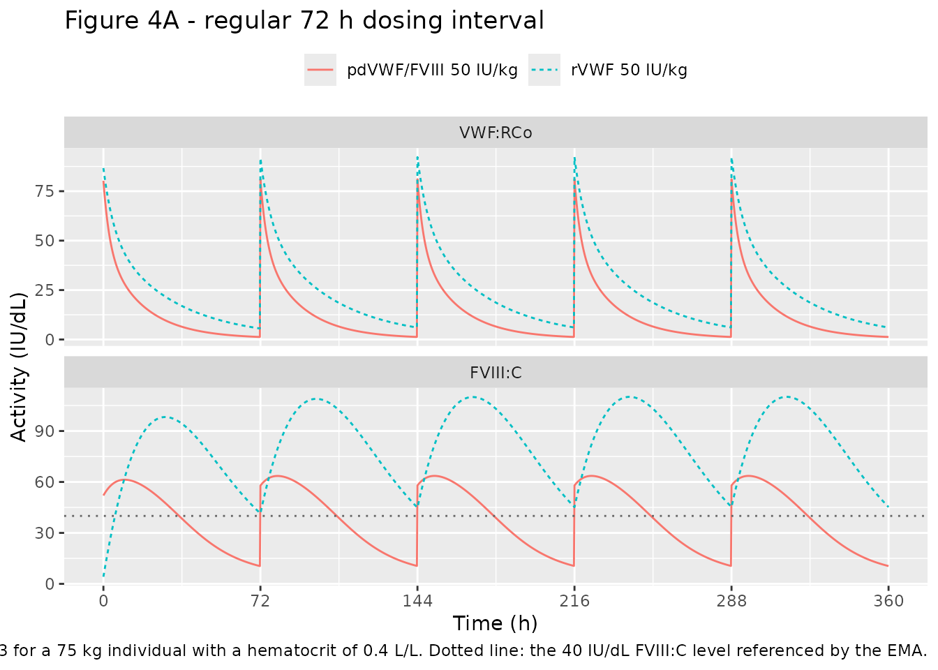

The paper’s headline simulation claim is that “following repeated administration of rVWF (50 IU/kg), a FVIII:C activity of >40 IU/dL can be maintained for the full 72 h dosing interval”. The steady-state interval of the replication is summarised below.

ss_summary <- typ_reg |>
  filter(time >= 288, time <= 360) |>
  group_by(treatment) |>
  summarise(
    `VWF:RCo Cmax` = max(Cc),
    `VWF:RCo trough` = min(Cc),
    `FVIII:C Cmax` = max(Cfviii),
    `FVIII:C trough` = min(Cfviii),
    `% interval FVIII:C > 40 IU/dL` = 100 * mean(Cfviii > 40),
    .groups = "drop"
  )

ss_summary |>
  rename("Treatment" = treatment) |>
  knitr::kable(
    digits = 1,
    caption = paste(
      "Steady-state dosing interval (288-360 h) of the typical-patient",
      "replication of Figure 4A."
    )
  )

Steady-state dosing interval (288-360 h) of the typical-patient replication of Figure 4A.
Treatment	VWF:RCo Cmax	VWF:RCo trough	FVIII:C Cmax	FVIII:C trough	% interval FVIII:C > 40 IU/dL
pdVWF/FVIII 50 IU/kg	81.1	1.3	63.6	10.5	48.8
rVWF 50 IU/kg	92.3	6.1	110.1	45.2	100.0

# Replicates Figure 4B of Bauer 2023: irregular 72 h / 96 h dosing intervals.
dose_times_irr <- cumsum(c(0, rep(c(72, 96), times = 3)))
grid_irr <- sort(unique(c(seq(0, max(dose_times_irr) + 96, by = 0.25), dose_times_irr)))

typ_irr <- bind_rows(
  solve_typical(mod_rvwf, vwf_doses(dose_times_irr), grid_irr) |>
    mutate(treatment = "rVWF 50 IU/kg"),
  solve_typical(
    mod_pd,
    bind_rows(vwf_doses(dose_times_irr), fviii_doses(dose_times_irr)),
    grid_irr
  ) |>
    mutate(treatment = "pdVWF/FVIII 50 IU/kg")
)

typ_irr |>
  select(time, treatment, `VWF:RCo` = Cc, `FVIII:C` = Cfviii) |>
  pivot_longer(c(`VWF:RCo`, `FVIII:C`), names_to = "analyte", values_to = "activity") |>
  mutate(analyte = factor(analyte, levels = c("VWF:RCo", "FVIII:C"))) |>
  ggplot(aes(time, activity, colour = treatment, linetype = treatment)) +
  geom_line() +
  geom_hline(
    data = data.frame(analyte = factor("FVIII:C", levels = c("VWF:RCo", "FVIII:C"))),
    aes(yintercept = 40), linetype = "dotted", colour = "grey40"
  ) +
  geom_vline(xintercept = dose_times_irr, colour = "grey85", linewidth = 0.2) +
  facet_wrap(~analyte, ncol = 1, scales = "free_y") +
  labs(
    x = "Time (h)", y = "Activity (IU/dL)", colour = NULL, linetype = NULL,
    title = "Figure 4B - irregular 72 h / 96 h dosing intervals",
    caption = paste(
      "Replicates Figure 4B of Bauer 2023. As the paper reports, only the",
      "troughs of the 96 h intervals fall below 40 IU/dL for rVWF."
    )
  ) +
  theme(legend.position = "top")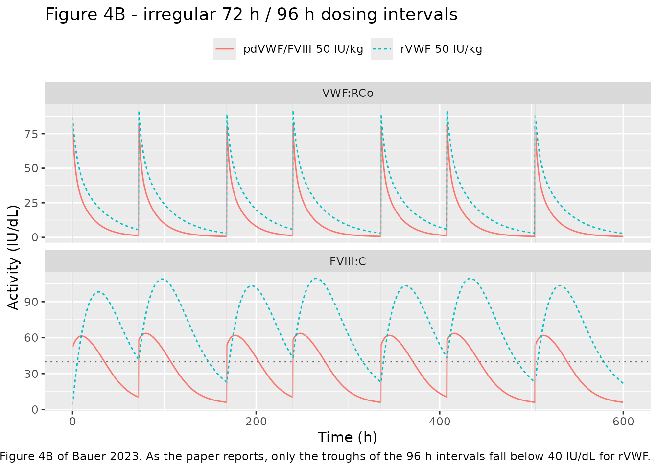

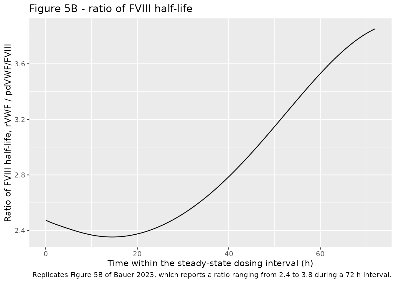
Figure 5 plots the model-predicted FVIII half-life during a steady-state dosing interval, and its rVWF-to-pdVWF/FVIII ratio. Because VWF:RCo inhibits kout, the FVIII half-life is time-varying within the interval: t1/2 = ln(2) / (kout * VWF effect). Both kout and vwfEffect are returned as columns by rxSolve.

# Replicates Figures 5A and 5B of Bauer 2023.
half_life <- typ_reg |>
  filter(time >= 288, time <= 360) |>
  mutate(
    time_in_interval = time - 288,
    fviii_half_life = log(2) / (kout * vwfEffect)
  ) |>
  select(time_in_interval, treatment, fviii_half_life)

ratio <- half_life |>
  pivot_wider(names_from = treatment, values_from = fviii_half_life) |>
  mutate(ratio = `rVWF 50 IU/kg` / `pdVWF/FVIII 50 IU/kg`)

ggplot(half_life, aes(time_in_interval, fviii_half_life,
                      colour = treatment, linetype = treatment)) +
  geom_line() +
  labs(
    x = "Time within the steady-state dosing interval (h)",
    y = "FVIII half-life (h)", colour = NULL, linetype = NULL,
    title = "Figure 5A - model-predicted FVIII half-life",
    caption = "Replicates Figure 5A of Bauer 2023."
  ) +
  theme(legend.position = "top")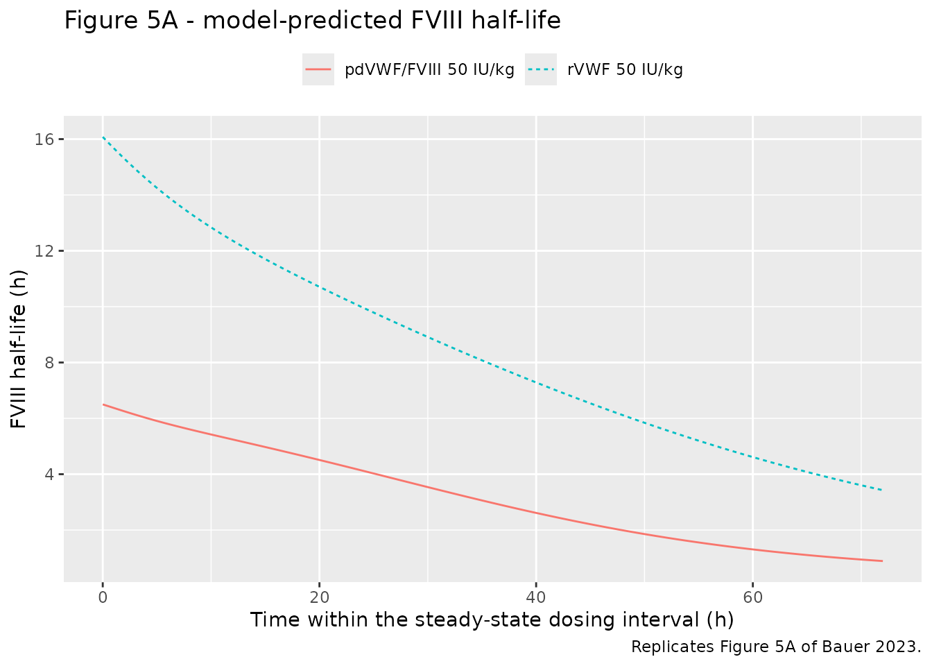


ggplot(ratio, aes(time_in_interval, ratio)) +
  geom_line() +
  labs(
    x = "Time within the steady-state dosing interval (h)",
    y = "Ratio of FVIII half-life, rVWF / pdVWF/FVIII",
    title = "Figure 5B - ratio of FVIII half-life",
    caption = paste(
      "Replicates Figure 5B of Bauer 2023, which reports a ratio ranging",
      "from 2.4 to 3.8 during a 72 h interval."
    )
  )

tibble::tibble(
  Quantity = "Ratio of FVIII half-life (rVWF / pdVWF/FVIII) over the 72 h interval",
  Simulated = sprintf("%.2f - %.2f", min(ratio$ratio), max(ratio$ratio)),
  Published = "2.4 - 3.8"
) |>
  knitr::kable(caption = "Bauer 2023 Figure 5B and text.")

Bauer 2023 Figure 5B and text.
Quantity	Simulated	Published
Ratio of FVIII half-life (rVWF / pdVWF/FVIII) over the 72 h interval	2.35 - 3.85	2.4 - 3.8

Virtual cohort

Original observed data are not publicly available. The stochastic simulation below uses virtual populations whose body-weight and hematocrit distributions approximate the published demographics: median 72.5 kg (range 45-143) and hematocrit 0.402 L/L (range 0.31-0.48) for the rVWF FVIII PK/PD population (Table 2), and median 66.3 kg (range 43.8-132) and hematocrit 0.406 L/L (range 0.334-0.483) for the pdVWF/FVIII population (Table 3). Weight is drawn log-normally and hematocrit normally, both truncated to the published range; the paper reports only medians and ranges, so the dispersion is an assumption (see Assumptions and deviations).

set.seed(20230612)

N_PER_ARM <- 150  # <= 200 per arm

make_arm <- function(n, treatment, wt_med, wt_lo, wt_hi,
                     hct_med, hct_lo, hct_hi, id_offset = 0L) {
  tibble::tibble(
    id        = id_offset + seq_len(n),
    treatment = treatment,
    WT        = pmin(pmax(stats::rlnorm(n, log(wt_med), 0.27), wt_lo), wt_hi),
    HCT       = pmin(pmax(stats::rnorm(n, hct_med, 3.6), hct_lo), hct_hi)
  )
}

obs_times <- seq(0, 96, by = 1)

expand_arm <- function(subj, with_fviii_dose) {
  doses <- subj |>
    mutate(time = 0, amt = 50 * WT, evid = 1L, cmt = "central", dvid = 1L)
  if (with_fviii_dose) {
    doses <- bind_rows(
      doses,
      subj |>
        mutate(time = 0, amt = 50 * WT / 2.4, evid = 1L, cmt = "fviii", dvid = 1L)
    )
  }
  obs <- subj |>
    tidyr::crossing(time = obs_times) |>
    mutate(amt = NA_real_, evid = 0L, cmt = "central", dvid = 1L)
  bind_rows(doses, obs) |> arrange(id, time, desc(evid))
}

subj_rvwf <- make_arm(N_PER_ARM, "rVWF 50 IU/kg",
                      72.5, 45, 143, 40.2, 31.0, 48.0, id_offset = 0L)
subj_pd   <- make_arm(N_PER_ARM, "pdVWF/FVIII 50 IU/kg",
                      66.3, 43.8, 132, 40.6, 33.4, 48.3, id_offset = 1000L)

ev_rvwf <- expand_arm(subj_rvwf, with_fviii_dose = FALSE)
ev_pd   <- expand_arm(subj_pd,   with_fviii_dose = TRUE)

stopifnot(!anyDuplicated(unique(ev_rvwf[, c("id", "time", "evid", "cmt")])))
stopifnot(!anyDuplicated(unique(ev_pd[, c("id", "time", "evid", "cmt")])))
stopifnot(length(intersect(subj_rvwf$id, subj_pd$id)) == 0L)

Simulation

sim <- bind_rows(
  rxode2::rxSolve(mod_rvwf, ev_rvwf, keep = c("treatment", "WT", "HCT")) |>
    as.data.frame(),
  rxode2::rxSolve(mod_pd, ev_pd, keep = c("treatment", "WT", "HCT")) |>
    as.data.frame()
)

nrow(sim)
#> [1] 29100

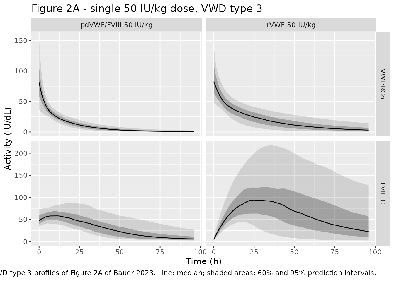
# Replicates the VWD type 3 panel of Figure 2A of Bauer 2023: simulated
# VWF:RCo and FVIII activity-time profiles following a single 50 IU/kg dose,
# with the 60% and 95% prediction intervals.
sim |>
  select(time, treatment, `VWF:RCo` = Cc, `FVIII:C` = Cfviii) |>
  pivot_longer(c(`VWF:RCo`, `FVIII:C`), names_to = "analyte", values_to = "activity") |>
  mutate(analyte = factor(analyte, levels = c("VWF:RCo", "FVIII:C"))) |>
  group_by(time, treatment, analyte) |>
  summarise(
    Q025 = quantile(activity, 0.025),
    Q20  = quantile(activity, 0.20),
    Q50  = quantile(activity, 0.50),
    Q80  = quantile(activity, 0.80),
    Q975 = quantile(activity, 0.975),
    .groups = "drop"
  ) |>
  ggplot(aes(time, Q50)) +
  geom_ribbon(aes(ymin = Q025, ymax = Q975), alpha = 0.15) +
  geom_ribbon(aes(ymin = Q20, ymax = Q80), alpha = 0.30) +
  geom_line() +
  facet_grid(analyte ~ treatment, scales = "free_y") +
  labs(
    x = "Time (h)", y = "Activity (IU/dL)",
    title = "Figure 2A - single 50 IU/kg dose, VWD type 3",
    caption = paste(
      "Replicates the VWD type 3 profiles of Figure 2A of Bauer 2023.",
      "Line: median; shaded areas: 60% and 95% prediction intervals."
    )
  )

PKNCA validation

VWF:RCo, typical patient

VWF:RCo is the dosed analyte, so NCA is run on it. Two points of care:

The model carries a non-decaying endogenous background E_VWF = 0.5 IU/dL. Leaving it in place would bias the terminal slope and make aucinf.obs diverge, so the NCA is run on the baseline-corrected exogenous activity, which is the standard convention for coagulation-factor NCA. E_VWF is the same fixed 0.5 IU/dL in both models.
The values reported in Table 4 are those of the reference patient (75 kg, hematocrit 0.4 L/L), at which every covariate factor equals 1. The comparison against them is therefore run on a typical-value single-dose profile with variability switched off and a fine observation grid, so that neither between-subject variability nor trapezoidal discretisation contaminates the check.

E_VWF <- 0.5
grid_nca <- sort(unique(c(seq(0, 240, by = 0.1))))

typ_single <- bind_rows(
  solve_typical(mod_rvwf, vwf_doses(0), grid_nca) |>
    mutate(treatment = "rVWF 50 IU/kg"),
  solve_typical(mod_pd, bind_rows(vwf_doses(0), fviii_doses(0)), grid_nca) |>
    mutate(treatment = "pdVWF/FVIII 50 IU/kg")
) |>
  mutate(id = 1L)

nca_typ_conc <- typ_single |>
  filter(!is.na(Cc)) |>
  mutate(Cc = pmax(Cc - E_VWF, 0)) |>
  select(id, time, Cc, treatment)

# Guarantee a time = 0 record. For an IV bolus the natural t = 0 row already
# holds dose/Vc, so the existing row wins via .keep_all = TRUE.
nca_typ_conc <- bind_rows(
  nca_typ_conc,
  nca_typ_conc |> distinct(id, treatment) |> mutate(time = 0, Cc = 0)
) |>
  distinct(id, treatment, time, .keep_all = TRUE) |>
  arrange(id, treatment, time)

nca_typ_dose <- tibble::tibble(
  id = 1L, time = 0, amt = 50 * WT_TYP,
  treatment = c("rVWF 50 IU/kg", "pdVWF/FVIII 50 IU/kg")
)

# Intravenous bolus: duration 0 so PKNCA does not offset the MRT estimate.
intervals_vwf <- data.frame(
  start = 0, end = Inf,
  cmax = TRUE, tmax = TRUE, aucinf.obs = TRUE,
  half.life = TRUE, mrt.iv.obs = TRUE, cl.obs = TRUE
)

nca_vwf_typ <- PKNCA::pk.nca(
  PKNCA::PKNCAdata(
    PKNCA::PKNCAconc(nca_typ_conc, Cc ~ time | treatment + id),
    PKNCA::PKNCAdose(
      nca_typ_dose, amt ~ time | treatment + id,
      route = "intravascular", duration = 0
    ),
    intervals = intervals_vwf
  )
)

VWF:RCo, virtual cohort

The same NCA run across the virtual cohort shows the spread the model implies. No published values exist to compare these against; they are reported so the population behaviour is visible.

sim_nca <- sim |>
  filter(!is.na(Cc)) |>
  mutate(Cc = pmax(Cc - E_VWF, 0)) |>
  select(id, time, Cc, treatment)

sim_nca <- bind_rows(
  sim_nca,
  sim_nca |> distinct(id, treatment) |> mutate(time = 0, Cc = 0)
) |>
  distinct(id, treatment, time, .keep_all = TRUE) |>
  arrange(id, treatment, time)

dose_df <- bind_rows(ev_rvwf, ev_pd) |>
  filter(evid == 1, cmt == "central") |>
  select(id, time, amt, treatment)

dose_obj <- PKNCA::PKNCAdose(
  dose_df, amt ~ time | treatment + id,
  route = "intravascular", duration = 0
)

nca_vwf_pop <- PKNCA::pk.nca(
  PKNCA::PKNCAdata(
    PKNCA::PKNCAconc(sim_nca, Cc ~ time | treatment + id),
    dose_obj,
    intervals = intervals_vwf
  )
)

as.data.frame(nca_vwf_pop) |>
  filter(PPTESTCD %in% c("cmax", "aucinf.obs", "half.life", "cl.obs")) |>
  group_by(treatment, PPTESTCD) |>
  summarise(
    summary = sprintf("%.1f (%.1f - %.1f)", median(PPORRES),
                      quantile(PPORRES, 0.05), quantile(PPORRES, 0.95)),
    .groups = "drop"
  ) |>
  pivot_wider(names_from = PPTESTCD, values_from = summary) |>
  rename(
    "Treatment" = treatment,
    "Cmax (IU/dL)" = cmax,
    "AUC0-inf (IU*h/dL)" = aucinf.obs,
    "t1/2 (h)" = half.life,
    "CL (dL/h)" = cl.obs
  ) |>
  knitr::kable(
    caption = paste(
      "Simulated single-dose VWF:RCo NCA across the virtual cohort:",
      "median (5th - 95th percentile). Baseline-corrected for E_VWF."
    )
  )

Simulated single-dose VWF:RCo NCA across the virtual cohort: median (5th - 95th percentile). Baseline-corrected for E_VWF.
Treatment	AUC0-inf (IU*h/dL)	CL (dL/h)	Cmax (IU/dL)	t1/2 (h)
pdVWF/FVIII 50 IU/kg	892.1 (616.5 - 1321.1)	3.9 (2.4 - 6.0)	80.9 (41.1 - 130.6)	12.3 (7.8 - 20.1)
rVWF 50 IU/kg	1894.1 (868.4 - 3454.0)	2.0 (1.0 - 4.3)	82.3 (50.5 - 131.3)	22.3 (10.7 - 43.8)

FVIII:C

The paper summarises FVIII exposure as AUC during the dosing interval (AUC72) and maximum activity (Cmax) (Figure 2C and 2D), so the FVIII:C block computes those over 0-72 h on the uncorrected activity.

sim_nca_fviii <- sim |>
  filter(!is.na(Cfviii)) |>
  select(id, time, Cc = Cfviii, treatment)

conc_fviii <- PKNCA::PKNCAconc(sim_nca_fviii, Cc ~ time | treatment + id)

intervals_fviii <- data.frame(
  start = 0, end = 72,
  cmax = TRUE, tmax = TRUE, auclast = TRUE
)

nca_fviii <- PKNCA::pk.nca(
  PKNCA::PKNCAdata(conc_fviii, dose_obj, intervals = intervals_fviii)
)

as.data.frame(nca_fviii) |>
  filter(PPTESTCD %in% c("cmax", "tmax", "auclast")) |>
  group_by(treatment, PPTESTCD) |>
  summarise(median = median(PPORRES), .groups = "drop") |>
  pivot_wider(names_from = PPTESTCD, values_from = median) |>
  rename(
    "Treatment" = treatment,
    "FVIII:C Cmax (IU/dL)" = cmax,
    "FVIII:C Tmax (h)" = tmax,
    "FVIII:C AUC72 (IU*h/dL)" = auclast
  ) |>
  knitr::kable(
    digits = 1,
    caption = paste(
      "Simulated single-dose FVIII exposure over the 72 h dosing interval,",
      "medians across the virtual cohort. Bauer 2023 reports the",
      "corresponding summary statistics only inside the panels of Figure 2C",
      "and 2D, so no numeric comparison is possible."
    )
  )

Simulated single-dose FVIII exposure over the 72 h dosing interval, medians across the virtual cohort. Bauer 2023 reports the corresponding summary statistics only inside the panels of Figure 2C and 2D, so no numeric comparison is possible.
Treatment	FVIII:C AUC72 (IU*h/dL)	FVIII:C Cmax (IU/dL)	FVIII:C Tmax (h)
pdVWF/FVIII 50 IU/kg	2555.6	60.7	9
rVWF 50 IU/kg	5120.0	95.5	28

Comparison against published values

Bauer 2023 does not tabulate NCA parameters for either product. What it does report numerically are the primary PK parameter estimates (Table 4) and the rVWF-to-pdVWF/FVIII ratios of mean residence time, half-life and AUC0-inf (Results, PK Model for pdVWF/FVIII). The reference column below is therefore computed analytically from the Table 4 estimates, which for a linear two-compartment IV bolus in the reference patient are exact: Cmax = Dose / Vc, AUC0-inf = Dose / CL, CL = CL, MRT = (Vc + Vp) / CL, and the terminal half-life from the smaller eigenvalue of the disposition matrix. Agreement therefore confirms that the packaged ODE implementation reproduces the published parameterisation, rather than merely running.

analytic <- function(cl, vc, q, vp, dose) {
  k10 <- cl / vc; k12 <- q / vc; k21 <- q / vp
  a <- k10 + k12 + k21
  lambda_z <- (a - sqrt(a^2 - 4 * k10 * k21)) / 2
  c(
    cmax       = dose / vc,
    tmax       = 0,
    aucinf.obs = dose / cl,
    half.life  = log(2) / lambda_z,
    mrt.iv.obs = (vc + vp) / cl,
    cl.obs     = cl
  )
}

dose_typ <- 50 * WT_TYP  # 50 IU/kg in the 75 kg reference patient

published <- bind_rows(
  tibble::tibble(treatment = "rVWF 50 IU/kg",
                 !!!as.list(analytic(2.10, 43.5, 2.29, 15.8, dose_typ))),
  tibble::tibble(treatment = "pdVWF/FVIII 50 IU/kg",
                 !!!as.list(analytic(4.14, 47.0, 4.47, 19.3, dose_typ)))
)

cmp <- nlmixr2lib::ncaComparisonTable(
  simulated = nca_vwf_typ,
  reference = published,
  by        = "treatment",
  units     = c(cmax = "IU/dL", tmax = "h", aucinf.obs = "IU*h/dL",
                half.life = "h", mrt.iv.obs = "h", cl.obs = "dL/h"),
  tolerance_pct = 20
)

knitr::kable(
  cmp,
  digits  = 3,
  caption = paste(
    "Typical-patient simulated VWF:RCo NCA vs the values implied analytically",
    "by the Bauer 2023 Table 4 estimates. * differs from reference by >20%."
  )
)

Typical-patient simulated VWF:RCo NCA vs the values implied analytically by the Bauer 2023 Table 4 estimates. * differs from reference by >20%.
NCA parameter	treatment	Reference	Simulated	% diff
Cmax (IU/dL)	rVWF 50 IU/kg	86.2	86.2	+0.0%
Cmax (IU/dL)	pdVWF/FVIII 50 IU/kg	79.8	79.8	+0.0%
Tmax (h)	rVWF 50 IU/kg	0	0	—
Tmax (h)	pdVWF/FVIII 50 IU/kg	0	0	—
AUC0-∞ (obs) (IU*h/dL)	rVWF 50 IU/kg	1790	1790	+0.0%
AUC0-∞ (obs) (IU*h/dL)	pdVWF/FVIII 50 IU/kg	906	906	+0.0%
t½ (h)	rVWF 50 IU/kg	21.1	21	-0.4%
t½ (h)	pdVWF/FVIII 50 IU/kg	12.2	12.1	-0.3%
CL/F (dL/h)	rVWF 50 IU/kg	2.1	2.1	-0.0%
CL/F (dL/h)	pdVWF/FVIII 50 IU/kg	4.14	4.14	-0.0%
MRT (IV) (h)	rVWF 50 IU/kg	28.2	28.2	-0.0%
MRT (IV) (h)	pdVWF/FVIII 50 IU/kg	16	16	-0.0%

The three ratios the paper reports directly:

ratio_sim <- as.data.frame(nca_vwf_typ) |>
  filter(PPTESTCD %in% c("mrt.iv.obs", "half.life", "aucinf.obs")) |>
  select(treatment, PPTESTCD, PPORRES) |>
  pivot_wider(names_from = treatment, values_from = PPORRES) |>
  mutate(Simulated = `rVWF 50 IU/kg` / `pdVWF/FVIII 50 IU/kg`)

ratio_pub <- tibble::tribble(
  ~PPTESTCD,     ~Quantity,                    ~Published,
  "mrt.iv.obs",  "Mean residence time ratio",  1.76,
  "half.life",   "Terminal half-life ratio",   1.74,
  "aucinf.obs",  "AUC0-inf ratio",             1.97
)

ratio_pub |>
  left_join(ratio_sim |> select(PPTESTCD, Simulated), by = "PPTESTCD") |>
  mutate(`Difference (%)` = 100 * (Simulated - Published) / Published) |>
  select(Quantity, Simulated, Published, `Difference (%)`) |>
  knitr::kable(
    digits  = 2,
    caption = paste(
      "rVWF-to-pdVWF/FVIII ratios of VWF:RCo exposure, typical patient.",
      "Published values from Bauer 2023 Results, PK Model for pdVWF/FVIII."
    )
  )

rVWF-to-pdVWF/FVIII ratios of VWF:RCo exposure, typical patient. Published values from Bauer 2023 Results, PK Model for pdVWF/FVIII.
Quantity	Simulated	Published	Difference (%)
Mean residence time ratio	1.76	1.76	0.19
Terminal half-life ratio	1.73	1.74	-0.33
AUC0-inf ratio	1.97	1.97	0.07

Both products were dosed at 50 IU/kg VWF:RCo in the same reference patient, so the AUC0-inf ratio reduces to the clearance ratio 4.14 / 2.10 = 1.97 exactly, and the MRT and half-life ratios follow from the four disposition parameters alone.

Assumptions and deviations

Initial condition of the FVIII pool. The paper defines FVIII0 as the FVIII:C level at VWF:RCo = 0 IU/dL and derives kin = FVIII0 * kout from the steady-state condition, but does not state the pre-dose initial condition. A VWD type 3 patient carries the endogenous E_VWF = 0.5 IU/dL, at which the VWF effect is already 0.118, so FVIII0 itself is not a steady state of the system. Both model files therefore initialise the pool at the drug-free steady state implied by E_VWF, fviii(0) = FVIII0_i / (1 - Imax * E_VWF / (IC50 + E_VWF)), which for the typical patient is 4.17 IU/dL. Initialising at FVIII0 instead would make FVIII:C drift upward before the first dose, which no figure in the paper shows.
Hematocrit unit. The paper reports hematocrit in L/L; the canonical covariate unit in nlmixr2lib is percent. The reference values 0.4 and 0.39 L/L are encoded as 40 and 39 %. The power ratio is unit-invariant provided the supplied HCT column uses the same unit as the reference.
Intravenous dosing represented as a bolus. The paper describes intravenous infusion but does not report an infusion duration, so doses are encoded as bolus inputs. This affects only the first minutes of each profile.
Imax rounding. The FVIII half-life is extremely sensitive to Imax because the effective removal rate is kout * (1 - Imax * ...) and Imax is reported to three significant figures (0.998, 1 - Imax = 0.002). Using the reported 0.998 with the reported kout = 15.9 1/h at VWF:RCo = 50 IU/dL gives an adjusted kout of 0.053 1/h and an FVIII half-life of 13.2 h, whereas the paper’s Supplementary Results quote 0.06 1/h and 11.5 h (95% CI 10.1-13.3 h) for the same calculation. The simulated value falls inside the published CI, and the paper’s point estimate is recovered with Imax = 0.9975 – i.e. the discrepancy is the rounding of the published Imax, not a structural difference. Absolute FVIII:C predictions should be read with this in mind; the ratio comparisons in Figure 5 are unaffected because both products carry the same sensitivity.
VWD type 3 parameterisation only. The rVWF VWF:RCo PK model was fitted across VWD types 1, 2, 3 and severe hemophilia A, with the typical endogenous VWF level entering as a structural covariate on disease group. Table 4 reports only the VWD type 3 value (0.500 IU/dL, fixed at half the LLOQ); the values for non-type-3 VWD and for severe hemophilia A are not reported in the paper or its supplement. Both model files therefore encode the VWD type 3 parameterisation, which is also the population the paper simulates. To model a patient with no endogenous VWF at all, set bl_vwf to 0.
Interindividual variability on E_VWF omitted. The paper states that the variability in endogenous VWF differed between patient populations but was set to 0 for VWD type 3, because only about 9% (5/57) of type 3 patients had estimated endogenous levels above the LLOQ. bl_vwf therefore carries no eta.
IIV magnitudes converted from CV. Table 4 reports the IIV magnitudes as
1. The Supplementary Methods specify an exponential IIV model P_i = TVP * exp(eta_i), so the reported CVs are converted to log-scale variances with omega^2 = log(1 + CV^2). If the authors instead reported the standard deviations of the etas directly (the common CV% ~ omega approximation), the variances would be about 8% larger.
No interoccasion variability. Interoccasion variability was tested during model development (Supplementary Methods, Stochastic Model) but is not part of the final parameter set in Table 4, so it is not encoded.
Virtual-cohort covariate dispersion. The paper reports only medians and ranges for body weight and hematocrit. Weight is drawn log-normally (sdlog = 0.27) and hematocrit normally (sd = 3.6 %), both truncated to the published range. The dispersion is chosen so the simulated interquartile spread is plausible for the published range; it is not a published quantity.
Baseline-corrected NCA. The VWF:RCo NCA subtracts the fixed endogenous E_VWF = 0.5 IU/dL before computing the terminal slope and AUC. Without the correction the non-decaying background inflates aucinf.obs without bound.
No published NCA table to compare against. Bauer 2023 reports no NCA parameter table. The comparison table therefore uses reference values computed analytically from the Table 4 point estimates, and the ratio table uses the three ratios the paper reports in prose. All values in the comparison originate in the paper; none were tuned.
Covariates screened but not retained. Age, sex, race, disease type, blood group, rFVIII coadministration and hematocrit on Vp were screened in the stepwise covariate procedure (Supplementary Table 1) but not retained. They are recorded in each model file’s covariatesDataExcluded metadata rather than covariateData, since they are not referenced in model(). A formal covariate analysis was not possible at all for the pdVWF/FVIII model given n=20, so the rVWF covariates were carried over unchanged.