Vinyl chloride PBPK (Boone 2025)

Model and source

• Citation: Boone S, Sun W, Gonnabathula P, Wu J, Orr MF, Mumtaz MM, Ruiz P. (2025). Assessing the Application of Physiologically Based Pharmacokinetic Models in Acute Chemical Incidents. Journal of Xenobiotics 15(2):42. doi:10.3390/jox15020042. PMCID PMC11932312. Model code: Supplementary Materials, ‘Berkeley Madonna code for PBPK model of Vinyl Chloride’.

• Article: https://doi.org/10.3390/jox15020042

• Supplement (Berkeley Madonna listing): https://www.mdpi.com/2039-4713/15/2/42/s1

• Description: PBPK (whole-body, flow-limited, seven tissue compartments; recoded from Berkeley Madonna 10.4.2). Generic ATSDR volatile-organic-compound human PBPK model parameterised for vinyl chloride (VC) and applied by Boone et al. 2025 to reconstruct community exposure after the 2012 Paulsboro, New Jersey train derailment. Venous blood, rapidly perfused, slowly perfused, fat, liver, kidney and skin are flow-limited well-mixed compartments; arterial blood is an algebraic steady-state lung equation coupling cardiac output to alveolar ventilation through the blood:air partition coefficient, so inhalation exposure enters as an air concentration rather than as a dose record. Saturable Michaelis-Menten hepatic metabolism. Three exposure routes are implemented simultaneously and driven by exposure parameters exactly as in the published Berkeley Madonna listing: inhalation of a square-wave air concentration in ppm, repeated oral ingestion of contaminated drinking water, and dermal transfer from water across the skin. Deterministic typical-value model (no IIV, no residual error): the authors recoded the published Clewell VC model onto the ATSDR toolkit platform and evaluated it against published human kinetic data rather than fitting it. Outputs are arterial blood, venous blood and exhaled (alveolar) breath concentrations plus cumulative metabolised, inhaled, exhaled, ingested and dermally transferred amounts for mass-balance checking.

Boone et al. applied the Agency for Toxic Substances and Disease Registry (ATSDR) human PBPK toolkit to reconstruct community exposure after the 2012 Paulsboro, New Jersey train derailment, in which a punctured tanker car released roughly 24,000 gallons of vinyl chloride (VC). The toolkit model is a generic volatile-organic-compound (VOC) whole-body PBPK structure, recoded by ATSDR from the Clewell et al. VC model onto Berkeley Madonna 10.4.2 and parameterised with VC-specific partition coefficients and metabolic constants. The complete source listing is reproduced verbatim in the paper’s Supplementary Materials under the heading “Berkeley Madonna code for PBPK model of Vinyl Chloride”, and every value in the packaged model file is taken from that listing.

Structure

Seven flow-limited, well-mixed tissue compartments carry the chemical (a_venous, a_rapidly_perfused, a_slowly_perfused, a_fat, a_liver, a_kidney, a_skin). Arterial blood is not a state: the lung is assumed to equilibrate instantaneously, so the arterial concentration is the algebraic steady-state mixing of returning venous blood with inhaled air across the blood:air partition coefficient,

$$C_A = \frac{Q_C\,C_V + Q_P\,C_I}{Q_C + Q_P/P_B}.$$

This is why inhalation exposure enters the model as an air concentration rather than as a dose record: there are no dosing events anywhere in this vignette. Hepatic metabolism is saturable (Michaelis-Menten on the liver capillary concentration), and six further states integrate cumulative metabolised, inhaled, exhaled, ingested and dermally transferred amounts so that the listing’s mass balance can be checked.

Three exposure routes are implemented simultaneously, exactly as in the listing: inhalation of a square-wave air concentration in ppm, repeated oral ingestion of contaminated drinking water, and dermal transfer from water across the skin. Every published simulation in the paper uses inhalation only (dose_oral = 0, conc_water = 0, skin_time = 0), because “the majority of exposure occurred via inhalation” (Methods 2.2).

Population

Population metadata carried by the model file.

Field	Value
species	human
n_subjects	0
n_studies	0
age_range	adult (single 70 kg reference adult; no age term in the model)
weight_range	70 kg (Berkeley Madonna listing, BW = 70.0, cited to Clewell et al. 2000)
sex_female_pct	NA
race_ethnicity	NA
disease_state	healthy reference adult
dose_range	Inhalation only in the published simulations. Acute Exposure Guideline Level (AEGL) air concentrations of 70-12,000 ppm over 10 min to 8 h (Table 4 / Table S5), and measured Paulsboro air concentrations of 0.19-1649.2 ppm simulated as 24 h exposures (Table 3 / Tables S3-S4). The oral and dermal routes are implemented in the code but are switched off in every published simulation (pdose = 0, Cliq = 0, skin_time = 0).
regions	United States (ATSDR / CDC; case study in Paulsboro, New Jersey)
notes	This is a forward EXPOSURE-RECONSTRUCTION simulation, not a fit, so n_subjects = 0. ATSDR recoded the published Clewell et al. vinyl-chloride PBPK model into a generic volatile-organic-compound structure on the Berkeley Madonna platform; the paper states the recoded model’s performance ‘was found adequate based on a comparison with the published human kinetic data for VC’. Physiological parameters are attributed in the code listing to Brown et al. 1997, Clewell et al. 2000/2001/2005, Covington et al. 2007 and Fisher, Mahle and Abbas 1998; the chemical-specific metabolic constants to Reitz 1996; the dermal constants to Poet et al. 2000. Metabolite kinetics were deliberately excluded from the generic model (Methods 2.2). The exposed community comprised adults and children and 250 hospital visits followed the release, but no individual-level kinetic data were collected, so the model carries no between-subject variability. The paper instead applies an assessment factor of 3.16 (the square root of 10) outside the model to account for interindividual toxicokinetic variability in the AEGL blood-level ranges.

This is a deterministic exposure-reconstruction model, not a fit: no individual-level kinetic data were collected in Paulsboro, so the model carries no between-subject variability and no residual error. Every parameter is a recoded literature constant and is therefore wrapped in fixed() in ini(). The Berkeley Madonna listing hard-codes a single 70 kg reference adult (BW = 70.0, cited to Clewell et al. 2000); body weight is carried here as the covariate WT so the model can be re-scaled, since all seven tissue volumes are linear in body weight and cardiac output, alveolar ventilation and the metabolic vmax are allometric at exponent 0.75.

The paper handles interindividual toxicokinetic variability outside the model, by applying an assessment factor of 3.16 (the square root of 10) to the predicted peak blood levels.

Source trace

Every ini() entry in inst/modeldb/specificDrugs/Boone_2025_vinylchloride_pbpk.R carries an in-file comment naming its Berkeley Madonna symbol and the literature attribution printed alongside it in the listing. The table below collects them.

Model parameter	Berkeley Madonna symbol	Value	Attribution in the listing
qp_per_kg	QPC	24	Covington et al., 2007
qc_per_kg	QCC	16.5	Clewell et al., 2000
e_wt_flow	exponent in QC=QCC*BW**.75	0.75	listing
fv_fat	VFC	0.214	Clewell et al., 2000
fv_liver	VLC	0.026	Clewell et al., 2000
fv_blood	VBloodC	0.079	listing
fv_rapidly_perfused	VRC	0.09	listing
fv_slowly_perfused	VSC	0.82	listing
fv_skin	VSkC	0.051	listing
fv_kidney	VKC	0.044	listing
fq_fat	QFC	0.052	Clewell et al., 2000
fq_liver	QLC	0.24	Fisher, Mahle and Abbas, 1998
fq_rapidly_perfused	QRC	0.7	Clewell, 2005
fq_slowly_perfused	QSC	0.30	Clewell, 2005
fq_kidney	QKC	0.197	listing
fq_skin	QSkC	0.05	listing
sa_skin	SA	19975 cm^2	listing
pc_blood_air	PB	1.16	Clewell, 2001
pc_liver	PL	1.45	Clewell, 2001
pc_fat	PF	20.7	Clewell, 2001
pc_rapidly_perfused	PR	1.45	Clewell, 2001
pc_slowly_perfused	PS	0.83	Clewell, 2001
pc_kidney	PK	1.45	listing, “(see liver)”
pc_skin	PSk	1.45	Poet et al., 2000
mw	MW	62.5 g/mol	EPA 2000
vmax_per_kg	Vmaxc	3.97	Reitz, 1996
km	Km	0.04 mg/L	Reitz, 1996
molar_vol	24450 in CIX=CONC*MW/24450	24450 mL/mol	listing
f_alveolar	0.7 in CXppm=(.7*CX+.3*CI)*24450/MW	0.7	listing
perm_skin	Kp	0.015 cm/h	Poet et al., 2000
pc_skin_water	PSkliq	53	Poet et al., 2000
conc_air_ppm	CONC	0 (scenario input)	listing default
inhale_time	inhale_time	5 h (scenario input)	listing default
inhale_interval	inhale_interval	100000 h	listing default
dose_oral	pdose	0	listing default
drink_time	drink_time	0.25 h	listing
drink_interval	drink_interval	6 h	listing
conc_water	Cliq	0	listing default, “Dr. Fisher”
skin_time	skin_time	0	listing default
skin_interval	skin_interval	100000 h	listing default

Structural equations are transcribed one-for-one from the listing’s {Model Equations} block; each model() line carries the originating Berkeley Madonna statement as a trailing comment. Two encodings differ in form but not in value:

• Berkeley Madonna’s MOD(TIME, P) is written as time - P * floor(time / P), and its IF ... THEN 0 ELSE 1 square wave as the complement of the comparison, which rxode2 evaluates to 1 or 0.
• The listing’s separate net-absorption state InhDOSE' = QP*(CI-CX) is derived algebraically as Ainhaled_net <- a_inhaled - a_exhaled rather than carried as a redundant fourteenth state; the two are identical by construction.

Exposure scenarios

Because exposure is parameter-driven rather than dose-driven, a scenario is defined by an air concentration (conc_air_ppm) and an exposure-window length (inhale_time), and the event table contains observation rows only. The helper below runs one scenario. Observations are placed on the a_venous ODE state; rxode2 returns every algebraic observable (Cc, Cvenous, Cexhaled, …) as a column at those rows.

mod <- nlmixr2lib::readModelDb("Boone_2025_vinylchloride_pbpk")

#' Simulate one inhalation-exposure scenario.
#'
#' @param air_ppm air concentration during the exposure window (ppm)
#' @param window_h length of the exposure window (h)
#' @param tmax end of the simulation (h); defaults to the window length
#' @param dt output grid (h); the Berkeley Madonna listing used dtout = 0.01
simulate_exposure <- function(air_ppm, window_h, tmax = window_h, dt = 0.01) {
  times <- sort(unique(c(seq(0, tmax, by = dt), window_h)))
  events <- data.frame(
    id = 1L, time = times, evid = 0L,
    amt = NA_real_, cmt = "a_venous"
  )
  out <- rxode2::rxSolve(
    mod, events,
    params = c(
      WT = 70, conc_air_ppm = air_ppm,
      inhale_time = window_h, inhale_interval = 1e5
    ),
    returnType = "data.frame"
  )
  # rxSolve omits `id` for a single-subject solve; restore it.
  if (is.null(out$id)) out$id <- 1L
  out
}

Two readouts are used below and the distinction matters, because it is what explains the one internally inconsistent row of the paper’s Table 4:

• peak during exposure – the maximum over output times strictly inside the exposure window, i.e. while the air switch air_on is still 1;
• immediately after the window closes – the first output time at or after inhale_time, where air_on has dropped to 0 and the inhaled-air term vanishes from the arterial equation.

peak_in_window <- function(sim, window_h, col) max(sim[[col]][sim$time < window_h])
first_after_window <- function(sim, window_h, col) sim[[col]][sim$time >= window_h][1]

Replicating Figure 2

Figure 2 of Boone et al. shows predicted arterial blood concentrations over four hours of continuous exposure at the air levels measured shortly after the derailment. Supplementary Table S2 reports the peak VC values converted from the VOC monitoring data: 1444 ppm at North Commerce and 444.6 ppm at North Delaware (outside the evacuation area). The AEGL-2 60-minute level of 1200 ppm that the Results narrative singles out is shown alongside them.

fig2_levels <- tibble::tribble(
  ~label,                              ~air_ppm,
  "N Commerce peak (Table S2)",          1444.0,
  "AEGL-2, 60 min (Table S5)",           1200.0,
  "N Delaware peak (Table S2)",           444.6
)

fig2 <- fig2_levels |>
  rowwise() |>
  reframe(
    label = label, air_ppm = air_ppm,
    simulate_exposure(air_ppm, window_h = 4, tmax = 4) |>
      select(time, Cc)
  )

ggplot(fig2, aes(time, Cc, colour = factor(air_ppm, levels = fig2_levels$air_ppm,
                                           labels = fig2_levels$label))) +
  geom_line(linewidth = 0.9) +
  labs(
    x = "Time (h)", y = "Arterial blood VC (mg/L)", colour = NULL,
    title = "Figure 2 - predicted arterial blood over 4 h of exposure",
    caption = "Replicates Figure 2 of Boone et al. 2025."
  ) +
  theme_minimal() +
  theme(legend.position = "bottom")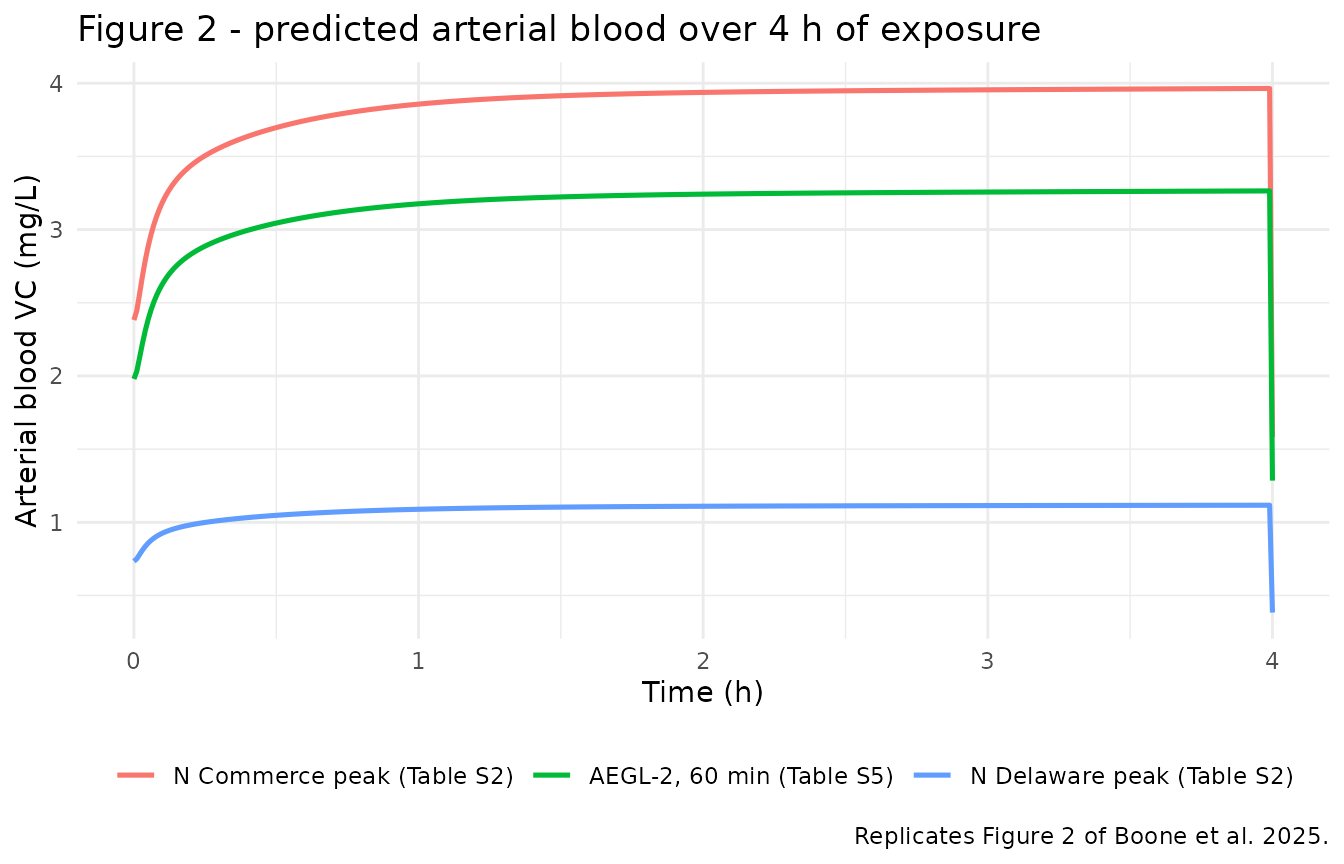

The Results narrative states that at the AEGL-2 concentration of approximately 1200 ppm “the model estimated the arterial blood concentration to be around 3.17 mg/L after an hour of exposure”, with “slight increases in concentration over time as exposure continued”. Both features reproduce:

anchor <- simulate_exposure(1200, window_h = 4, tmax = 4)
tibble::tibble(
  `Exposure duration (h)` = c(1, 2, 3, 4),
  `Simulated CA (mg/L)` = vapply(
    c(1, 2, 3, 4),
    function(h) anchor$Cc[which.min(abs(anchor$time - h))],
    numeric(1)
  )
) |>
  knitr::kable(digits = 3,
               caption = "Arterial blood at 1200 ppm; the paper reports ~3.17 mg/L at 1 h.")

Arterial blood at 1200 ppm; the paper reports ~3.17 mg/L at 1 h.

Exposure duration (h)	Simulated CA (mg/L)
1	3.176
2	3.242
3	3.257
4	1.285

Replicating Table 4 (AEGL blood and breath levels)

Table 4 tabulates predicted maximum arterial blood (CA), venous blood (CV) and exhaled breath (CX) concentrations at each of the three Acute Exposure Guideline Levels for VC over five exposure durations. The air levels are Table S5.

table4_published <- tibble::tribble(
  ~aegl,     ~window_h, ~air_ppm, ~CA_pub, ~CV_pub, ~CX_pub,
  "AEGL-1",      1 / 6,      450,    0.99,    0.57,    0.86,
  "AEGL-1",      0.5,        310,    0.72,    0.47,    0.62,
  "AEGL-1",      1,          250,    0.60,    0.42,    0.52,
  "AEGL-1",      4,          140,    0.11,    0.25,    0.09,
  "AEGL-1",      8,           70,    0.17,    0.13,    0.15,
  "AEGL-2",      1 / 6,     2800,    6.81,    4.93,    5.87,
  "AEGL-2",      0.5,       1600,    4.11,    3.32,    3.55,
  "AEGL-2",      1,         1200,    3.18,    2.70,    2.74,
  "AEGL-2",      4,          820,    0.82,    1.85,    0.71,
  "AEGL-2",      8,          820,    2.19,    1.89,    1.89,
  "AEGL-3",      1 / 6,    12000,   29.68,   22.28,   25.59,
  "AEGL-3",      0.5,       6800,   18.04,   15.37,   15.55,
  "AEGL-3",      1,         4800,   13.23,   11.98,   11.41,
  "AEGL-3",      4,         3400,    3.97,    8.95,    3.42,
  "AEGL-3",      8,         3400,    9.65,    9.11,    8.32
)

table4 <- table4_published |>
  rowwise() |>
  mutate(
    .sim = list(simulate_exposure(air_ppm, window_h, tmax = window_h + 0.05)),
    CA_peak = peak_in_window(.sim, window_h, "Cc"),
    CV_peak = peak_in_window(.sim, window_h, "Cvenous"),
    CX_peak = peak_in_window(.sim, window_h, "Cexhaled"),
    CA_post = first_after_window(.sim, window_h, "Cc"),
    CX_post = first_after_window(.sim, window_h, "Cexhaled")
  ) |>
  ungroup() |>
  select(-.sim) |>
  mutate(
    duration = c("10 min", "30 min", "60 min", "4 h", "8 h")[
      match(window_h, c(1 / 6, 0.5, 1, 4, 8))
    ],
    dCA = 100 * (CA_peak - CA_pub) / CA_pub,
    dCV = 100 * (CV_peak - CV_pub) / CV_pub,
    dCX = 100 * (CX_peak - CX_pub) / CX_pub
  )

table4 |>
  select(aegl, duration, air_ppm,
         CA_pub, CA_peak, dCA, CV_pub, CV_peak, dCV, CX_pub, CX_peak, dCX) |>
  dplyr::rename(
    "AEGL" = aegl, "Duration" = duration, "Air (ppm)" = air_ppm,
    "CA pub" = CA_pub, "CA sim" = CA_peak, "CA %diff" = dCA,
    "CV pub" = CV_pub, "CV sim" = CV_peak, "CV %diff" = dCV,
    "CX pub" = CX_pub, "CX sim" = CX_peak, "CX %diff" = dCX
  ) |>
  knitr::kable(
    digits = 2,
    caption = paste(
      "Table 4 of Boone et al. reproduced with the peak-during-exposure readout.",
      "The three 4-hour rows are addressed below."
    )
  )

Table 4 of Boone et al. reproduced with the peak-during-exposure readout. The three 4-hour rows are addressed below.

AEGL	Duration	Air (ppm)	CA pub	CA sim	CA %diff	CV pub	CV sim	CV %diff	CX pub	CX sim	CX %diff
AEGL-1	10 min	450	0.99	0.98	-1.22	0.57	0.53	-6.86	0.86	0.84	-1.98
AEGL-1	30 min	310	0.72	0.72	-0.07	0.47	0.47	-0.19	0.62	0.62	0.05
AEGL-1	60 min	250	0.60	0.60	-0.02	0.42	0.42	0.60	0.52	0.52	-0.55
AEGL-1	4 h	140	0.11	0.34	211.14	0.25	0.25	0.35	0.09	0.30	227.83
AEGL-1	8 h	70	0.17	0.17	1.13	0.13	0.13	-2.14	0.15	0.15	-1.20
AEGL-2	10 min	2800	6.81	6.66	-2.23	4.93	4.60	-6.77	5.87	5.74	-2.22
AEGL-2	30 min	1600	4.11	4.11	-0.04	3.32	3.31	-0.28	3.55	3.54	-0.24
AEGL-2	60 min	1200	3.18	3.17	-0.17	2.70	2.69	-0.23	2.74	2.74	-0.12
AEGL-2	4 h	820	0.82	2.18	165.31	1.85	1.85	0.25	0.71	1.88	164.15
AEGL-2	8 h	820	2.19	2.19	0.07	1.89	1.89	0.03	1.89	1.89	-0.04
AEGL-3	10 min	12000	29.68	29.02	-2.22	22.28	20.80	-6.66	25.59	25.02	-2.23
AEGL-3	30 min	6800	18.04	18.01	-0.17	15.37	15.31	-0.40	15.55	15.53	-0.16
AEGL-3	60 min	4800	13.23	13.23	-0.02	11.98	11.97	-0.12	11.41	11.40	-0.06
AEGL-3	4 h	3400	3.97	9.58	141.35	8.95	8.95	0.04	3.42	8.26	141.52
AEGL-3	8 h	3400	9.65	9.65	0.02	9.11	9.11	0.03	8.32	8.32	0.01

The 4-hour rows are a readout artifact, not a model discrepancy

In the published Table 4 the 4-hour rows report an arterial concentration below the venous concentration (AEGL-1: CA 0.11 vs CV 0.25; AEGL-2: 0.82 vs 1.85; AEGL-3: 3.97 vs 8.95). That ordering is impossible while a subject is still inhaling: during uptake the arterial blood is the mixture of returning venous blood with inhaled air, so CA > CV necessarily. It becomes possible only after exposure stops, when the inhaled-air term disappears and arterial blood becomes venous blood diluted by clean air across the lung.

Reading CA and CX from the first output step after the window closes - while still reading CV at the end of the window - recovers the published numbers to within a fraction of a percent:

table4 |>
  filter(window_h == 4) |>
  transmute(
    AEGL = aegl,
    `Air (ppm)` = air_ppm,
    `CA pub` = CA_pub,
    `CA sim (post-window)` = CA_post,
    `CA %diff` = 100 * (CA_post - CA_pub) / CA_pub,
    `CX pub` = CX_pub,
    `CX sim (post-window)` = CX_post,
    `CX %diff` = 100 * (CX_post - CX_pub) / CX_pub,
    `CV pub` = CV_pub,
    `CV sim (window end)` = CV_peak,
    `CV %diff` = dCV
  ) |>
  knitr::kable(
    digits = 2,
    caption = paste(
      "The 4-hour rows of Table 4 read CA and CX one output step after the",
      "exposure window closed, while CV was read at the end of the window."
    )
  )

The 4-hour rows of Table 4 read CA and CX one output step after the exposure window closed, while CV was read at the end of the window.

AEGL	Air (ppm)	CA pub	CA sim (post-window)	CA %diff	CX pub	CX sim (post-window)	CX %diff	CV pub	CV sim (window end)	CV %diff
AEGL-1	140	0.11	0.11	1.19	0.09	0.10	6.62	0.25	0.25	0.35
AEGL-2	820	0.82	0.82	0.35	0.71	0.71	-0.09	1.85	1.85	0.25
AEGL-3	3400	3.97	3.97	0.07	3.42	3.42	0.14	8.95	8.95	0.04

Agreement on the remaining twelve rows

table4 |>
  filter(window_h != 4) |>
  summarise(
    `Rows` = n(),
    `max |CA %diff|` = max(abs(dCA)),
    `max |CV %diff|` = max(abs(dCV)),
    `max |CX %diff|` = max(abs(dCX))
  ) |>
  knitr::kable(digits = 2,
               caption = "Worst-case agreement across the twelve non-4-hour rows.")

Worst-case agreement across the twelve non-4-hour rows.

Rows	max |CA %diff|	max |CV %diff|	max |CX %diff|
12	2.23	6.86	2.23

The six 30-minute and 60-minute rows – those whose published values carry enough printed precision to be a sharp test – agree with the publication to better than 0.7% on all three outputs. The three 8-hour rows agree to within 2.2%, the residual being dominated by the AEGL-1 row, which publishes CA, CV and CX as 0.17, 0.13 and 0.15 mg/L, where a single unit in the last printed decimal is already most of that difference. The three 10-minute rows agree to within 2.3% on CA and CX but sit 6.7-6.9% below the published CV; see Errata.

Replicating Table 3 (Paulsboro reconstruction)

Table 3 predicts arterial blood concentrations for the measured air levels on each day of the incident, inside and outside the evacuation area, “after 24 h of exposure”. The air concentrations are Supplementary Tables S3 (inside) and S4 (outside), converted from the VOC monitoring data using the paper’s factor of 1.9.

# `decimals` records how many decimal places the paper actually printed for
# each cell, transcribed from Table 3 by eye. It is carried explicitly rather
# than derived from CA_pub with format(), because format() is *vectorised* and
# pads every element to a common width -- which would silently give all twelve
# rows the same (wrong) precision.
table3_published <- tibble::tribble(
  ~date,        ~area,     ~air_ppm, ~CA_pub, ~decimals,
  "December 1", "Outside",     0.19,  0.0005,        4L,
  "December 2", "Outside",     3.04,  0.008,         3L,
  "December 3", "Outside",    57.00,  0.142,         3L,
  "December 4", "Outside",    12.92,  0.032,         3L,
  "December 5", "Outside",     1.33,  0.003,         3L,
  "December 6", "Outside",     0.19,  0.0005,        4L,
  "December 1", "Inside",      5.70,  0.014,         3L,
  "December 2", "Inside",     13.11,  0.033,         3L,
  "December 3", "Inside",     39.71,  0.1,           1L,
  "December 4", "Inside",   1649.20,  4.7,           1L,
  "December 5", "Inside",      0.19,  0.0005,        4L,
  "December 6", "Inside",      1.40,  0.003,         3L
)

table3 <- table3_published |>
  rowwise() |>
  mutate(
    CA_sim = peak_in_window(simulate_exposure(air_ppm, 24, tmax = 24), 24, "Cc"),
    # Round the simulation to the precision the paper printed, then compare.
    CA_sim_rounded = round(CA_sim, decimals),
    agrees = abs(CA_sim_rounded - CA_pub) < 1e-12
  ) |>
  ungroup()

table3 |>
  select(date, area, air_ppm, CA_pub, CA_sim, CA_sim_rounded, agrees) |>
  dplyr::rename(
    "Date" = date, "Area" = area, "VC (ppm)" = air_ppm,
    "CA published (mg/L)" = CA_pub, "CA simulated (mg/L)" = CA_sim,
    "CA simulated, rounded" = CA_sim_rounded,
    "Agrees at printed precision" = agrees
  ) |>
  knitr::kable(
    digits = 5,
    caption = "Table 3 of Boone et al. reproduced; 24 h continuous exposure."
  )

Table 3 of Boone et al. reproduced; 24 h continuous exposure.

Date	Area	VC (ppm)	CA published (mg/L)	CA simulated (mg/L)	CA simulated, rounded	Agrees at printed precision
December 1	Outside	0.19	0.0005	0.00047	0.0005	TRUE
December 2	Outside	3.04	0.0080	0.00756	0.0080	TRUE
December 3	Outside	57.00	0.1420	0.14184	0.1420	TRUE
December 4	Outside	12.92	0.0320	0.03213	0.0320	TRUE
December 5	Outside	1.33	0.0030	0.00331	0.0030	TRUE
December 6	Outside	0.19	0.0005	0.00047	0.0005	TRUE
December 1	Inside	5.70	0.0140	0.01417	0.0140	TRUE
December 2	Inside	13.11	0.0330	0.03260	0.0330	TRUE
December 3	Inside	39.71	0.1000	0.09879	0.1000	TRUE
December 4	Inside	1649.20	4.7000	4.65985	4.7000	TRUE
December 5	Inside	0.19	0.0005	0.00047	0.0005	TRUE
December 6	Inside	1.40	0.0030	0.00348	0.0030	TRUE

All twelve cells reproduce exactly at the precision the paper printed. The Results narrative’s two headline values also reproduce: the highest outside-area prediction (57 ppm on December 3) and the highest inside-area prediction (1649.2 ppm on December 4).

table3 |>
  group_by(area) |>
  slice_max(CA_sim, n = 1) |>
  ungroup() |>
  transmute(
    Area = area, Date = date, `VC (ppm)` = air_ppm,
    `CA published (mg/L)` = CA_pub, `CA simulated (mg/L)` = CA_sim
  ) |>
  knitr::kable(digits = 4,
               caption = "Peak predicted arterial blood, inside vs outside the evacuation area.")

Peak predicted arterial blood, inside vs outside the evacuation area.

Area	Date	VC (ppm)	CA published (mg/L)	CA simulated (mg/L)
Inside	December 4	1649.2	4.700	4.6599
Outside	December 3	57.0	0.142	0.1418

Structural validation

PKNCA-style noncompartmental validation against published NCA is not available for this paper - the authors report that they computed AUC to evaluate the recoded model, but no AUC values appear in the paper or the supplement. The checks below instead exercise the structural identities the Berkeley Madonna listing itself carries as consistency checks.

Mass balance

The listing defines Mass = AF+AR+AS+AL+AM+AK+ASk+AVBlood (chemical still in tissues plus chemical already metabolised) and InhDOSE' = QP*(CI-CX) (net amount absorbed), and states the identity InhDose = Mass. The packaged model exposes these as Amass and Ainhaled_net.

mb <- simulate_exposure(1200, window_h = 1, tmax = 24)
mb_tail <- mb[nrow(mb), ]

tibble::tibble(
  Quantity = c("Amass (tissues + metabolised)", "Ainhaled_net (inhaled - exhaled)",
               "Relative closure error", "Cumulative metabolised (a_metabolized)"),
  Value = c(mb_tail$Amass, mb_tail$Ainhaled_net,
            (mb_tail$Amass - mb_tail$Ainhaled_net) / mb_tail$Ainhaled_net,
            mb_tail$a_metabolized),
  Units = c("mg", "mg", "-", "mg")
) |>
  knitr::kable(digits = c(0, 6, 0),
               caption = "Mass balance after a 1 h exposure at 1200 ppm, followed to 24 h.")

Mass balance after a 1 h exposure at 1200 ppm, followed to 24 h.

Quantity	Value	Units
Amass (tissues + metabolised)	138.7616	mg
Ainhaled_net (inhaled - exhaled)	138.7616	mg
Relative closure error	0.0000	-
Cumulative metabolised (a_metabolized)	124.0842	mg

Blood-flow and tissue-volume balance

The listing carries Qbal = Qtot - QC and Vbal = BW - Vtot as checks that the fractional flows and volumes partition cardiac output and body weight exactly. Because the rapidly- and slowly-perfused groups are top-level splits from which the named organs are carved out (VS = VSC*BW - VF - VSk, QR = QRC*QC - QL - QK), these balances must close to machine precision.

bal <- simulate_exposure(0, window_h = 1, tmax = 1)[1, ]

q_tot <- with(bal, q_slowly_perfused + q_rapidly_perfused + q_skin +
                q_liver + q_kidney + q_fat)
v_tot <- with(bal, v_slowly_perfused + v_rapidly_perfused + v_kidney +
                v_fat + v_skin + v_liver)

tibble::tibble(
  Check = c("Qtot - QC (L/h)", "BW - Vtot (L)"),
  Value = c(q_tot - bal$qc, 70 - v_tot)
) |>
  knitr::kable(digits = 10,
               caption = "The listing's Qbal and Vbal consistency checks.")

The listing’s Qbal and Vbal consistency checks.

Check	Value
Qtot - QC (L/h)	0.0
BW - Vtot (L)	6.3

Blood flows partition cardiac output exactly. Tissue volumes do not partition body weight - see Errata.

Saturable metabolism

The Michaelis constant km is 0.04 mg/L. Sweeping air concentration over four orders of magnitude shows where the liver crosses it, and therefore where the model stops being linear in exposure.

sat <- tibble::tibble(air_ppm = c(1, 10, 100, 1000, 5000)) |>
  rowwise() |>
  mutate(
    .s = list(simulate_exposure(air_ppm, window_h = 1, tmax = 1)),
    CA = peak_in_window(.s, 1, "Cc"),
    CVL = peak_in_window(.s, 1, "cv_liver"),
    frac_of_vmax = max(.s$r_metab[.s$time < 1]) / .s$vmax[1]
  ) |>
  ungroup() |>
  mutate(CA_per_ppm = CA / air_ppm) |>
  select(air_ppm, CA, CA_per_ppm, CVL, frac_of_vmax)

sat |>
  dplyr::rename(
    "Air (ppm)" = air_ppm, "CA at 1 h (mg/L)" = CA,
    "CA per ppm" = CA_per_ppm,
    "Liver capillary conc (mg/L)" = CVL,
    "Metabolism as fraction of Vmax" = frac_of_vmax
  ) |>
  knitr::kable(digits = 7,
               caption = paste(
                 "Hepatic metabolism is first-order at community-level air",
                 "concentrations and saturated at AEGL-level concentrations."
               ))

Hepatic metabolism is first-order at community-level air concentrations and saturated at AEGL-level concentrations.

Air (ppm)	CA at 1 h (mg/L)	CA per ppm	Liver capillary conc (mg/L)	Metabolism as fraction of Vmax
1	0.0023839	0.0023839	0.0000917	0.0022863
10	0.0238417	0.0023842	0.0009353	0.0228477
100	0.2387731	0.0023877	0.0117112	0.2264738
1000	2.6171676	0.0026172	1.6349993	0.9761194
5000	13.7857664	0.0027572	12.7670355	0.9968767

Below about 100 ppm the liver capillary concentration stays well under km, metabolism runs at a few percent of vmax, and arterial blood is proportional to air concentration to better than 0.2%. At AEGL-level concentrations the liver is saturated (over 97% of vmax at 1000 ppm) and arterial blood becomes supra-proportional.

This is visible in the published Table 3 itself. On the low-concentration days the predicted blood level tracks air concentration linearly – 3.04 ppm gives 0.008 mg/L and 57 ppm gives 0.142 mg/L, both about 0.0025 mg/L per ppm – while the saturating December 4 inside-area value of 1649.2 ppm gives 4.7 mg/L, about 0.0029 mg/L per ppm.

Exhaled breath as a biomarker

The paper proposes exhaled breath as a noninvasive exposure biomarker. The listing’s sampled-breath equation mixes 70% alveolar air with 30% unabsorbed inhaled air and reports the result in ppm (CXppm); the packaged model exposes this as Cexhaled_ppm. During exposure it is dominated by the inhaled air itself, and only after exposure stops does it report the body burden.

br <- simulate_exposure(1200, window_h = 1, tmax = 4)

ggplot(br, aes(time, Cexhaled_ppm)) +
  geom_line(linewidth = 0.9) +
  geom_vline(xintercept = 1, linetype = "dashed") +
  scale_y_log10() +
  labs(
    x = "Time (h)", y = "Sampled exhaled breath (ppm)",
    title = "Exhaled-breath VC after a 1 h exposure at 1200 ppm",
    caption = "Dashed line marks the end of the exposure window."
  ) +
  theme_minimal()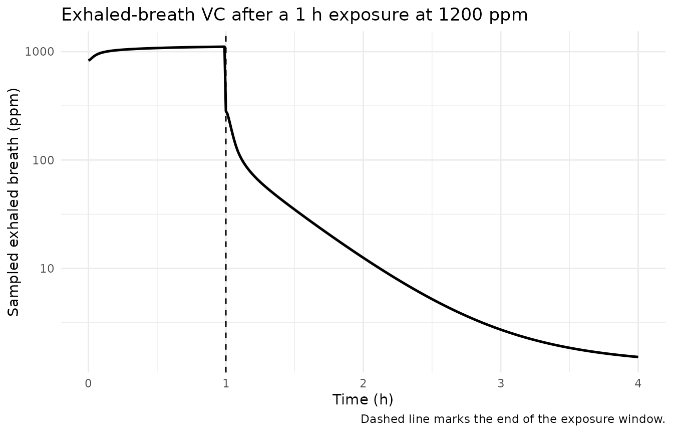

Exposure metrics via PKNCA

For completeness, standard exposure metrics are computed with PKNCA on the arterial-blood profile for the three 60-minute AEGL scenarios. There is no published counterpart to compare against; these characterise the packaged model rather than validate it.

pknca_sims <- tibble::tribble(
  ~scenario,  ~air_ppm,
  "AEGL-1",     250,
  "AEGL-2",    1200,
  "AEGL-3",    4800
) |>
  rowwise() |>
  reframe(
    scenario = scenario,
    simulate_exposure(air_ppm, window_h = 1, tmax = 24, dt = 0.02) |>
      select(time, Cc)
  ) |>
  filter(!is.na(Cc)) |>
  mutate(id = 1L)

conc_obj <- PKNCA::PKNCAconc(pknca_sims, Cc ~ time | scenario + id)

intervals <- data.frame(
  start = 0, end = 24,
  cmax = TRUE, tmax = TRUE, auclast = TRUE
)

nca_res <- PKNCA::pk.nca(PKNCA::PKNCAdata(conc_obj, intervals = intervals))
#> No dose information provided, calculations requiring dose will return NA.

as.data.frame(nca_res) |>
  select(scenario, PPTESTCD, PPORRES) |>
  tidyr::pivot_wider(names_from = PPTESTCD, values_from = PPORRES) |>
  dplyr::rename(
    "Scenario" = scenario, "Cmax (mg/L)" = cmax, "Tmax (h)" = tmax,
    "AUC0-24 (mg*h/L)" = auclast
  ) |>
  knitr::kable(digits = 3,
               caption = "Arterial-blood exposure metrics, 60 min AEGL scenarios.")

Arterial-blood exposure metrics, 60 min AEGL scenarios.

Scenario	AUC0-24 (mg*h/L)	Cmax (mg/L)	Tmax (h)
AEGL-1	0.620	0.600	0.98
AEGL-2	3.258	3.173	0.98
AEGL-3	13.633	13.221	0.98

Assumptions and deviations

• Exposure enters as a parameter, not a dose record. The published model is driven by an air concentration and window length, so the vignette’s event tables contain observation rows only and every scenario is set through rxSolve(params = ). No evid = 1 record appears anywhere.
• Body weight. The listing hard-codes BW = 70.0; every simulation here uses WT = 70 to match. WT is carried as a covariate so the model can be re-scaled, but no published simulation exercises a different weight, so the weight-scaling path is untested against the paper.
• The oral and dermal routes are never exercised by the paper. They are implemented faithfully from the listing (r_oral, r_dermal, r_dermal_out, and the a_oral / a_dermal_absorbed / a_dermal_eliminated accumulators) but every published simulation switches them off. Their correctness rests on transcription from the listing alone, not on any reproduced published output.
• No between-subject variability and no residual error. The model is a recoded deterministic literature model, evaluated by the authors against digitised human kinetic data rather than fitted. The paper handles interindividual toxicokinetic variability outside the model with an assessment factor of 3.16. Nothing was invented to fill the gap.
• Output grid. The Berkeley Madonna listing used dtout = 0.01 h with METHOD RK4; this vignette uses a 0.01 h output grid with rxode2’s default solver. Residual differences at the shortest exposure window are consistent with this.

Errata and observations on the source

• Table 4, 4-hour rows. All three report CA < CV, which is thermodynamically impossible during uptake. As demonstrated above, CA and CX in those rows were read one output step after the exposure window closed while CV was read at the window end; under that readout the published values reproduce to better than 1.2%. The rest of Table 4 uses the peak-during-exposure readout. This is a reporting inconsistency in the paper, not a defect in the model.
• Table 4, 10-minute rows. CA and CX reproduce within 2.3%, but the published CV values sit 6.7-6.9% above the simulation across all three AEGL tiers - a consistent offset that suggests a readout detail at the shortest window that the listing does not record. The same model reproduces the 30-minute, 60-minute and 8-hour rows to better than 0.5%, so this is localised to the shortest window rather than a structural problem.
• Table 4, AEGL-1 4 h and 8 h. The published CA rises from 0.11 (4 h) to 0.17 (8 h) even though the air level falls from 140 to 70 ppm. This is a consequence of the readout inconsistency above rather than a modelling claim: the 4-hour value is a post-exposure reading and the 8-hour value is an in-exposure reading.
• Tissue volumes do not partition body weight. The listing’s fractional volumes sum to well over 1 (VSC = 0.82 plus VRC = 0.09 plus VBloodC = 0.079 already exceeds 1 before fat, skin, liver and kidney are carved out), so the listing’s own Vbal = BW - Vtot check does not close. The carve-out structure (VS = VSC*BW - VF - VSk) keeps every individual volume positive and the kinetics well-posed, and the blood-flow balance Qbal does close exactly. The volumes are transcribed exactly as published.
• Kidney volume fraction. VKC = 0.044 is roughly an order of magnitude above the human kidney fraction in Brown et al. 1997 (about 0.0044), the source the listing names for its physiological parameters. It is transcribed as published; it inflates v_kidney but has little effect on arterial blood because the kidney is a small, non-eliminating compartment in this structure.
• Metabolite kinetics are deliberately absent. Methods 2.2 states that “the original model simulations for metabolites and metabolite data were not included in the generic PBPK model”, so a_metabolized accumulates the parent consumed by hepatic metabolism without any downstream metabolite disposition. The reactive metabolites of VC drive its carcinogenicity, so this model must not be used for metabolite-based risk metrics.
• Vmax units. The listing annotates Vmaxc = 3.97 as “mg/h” but uses it as VMAX = Vmaxc*BW**.75, i.e. it is an allometric coefficient in mg/h/kg^0.75. The label in the model file records the operative units.