Model and source
- Citation: Li M, Gao L, Wang Z, Zeng L, Chen C, Wang J, Li S, Liu M, Wang Y. Population pharmacokinetics and dose optimization of ceftazidime in critically ill children. Front Pharmacol. 2024;15:1470350. doi:10.3389/fphar.2024.1470350
- Description: One-compartment IV population PK model for ceftazidime in critically ill children (0.03-15 years) admitted to a paediatric intensive care unit (Li 2024). Clearance scales as a power function of body weight (exponent 0.90, reference 70 kg) and of modified-Schwartz estimated GFR (exponent 0.38, reference 116.93 mL/min/1.73 m^2); the volume of distribution scales linearly with body weight (exponent fixed to 1, reference 70 kg). Residual variability is additive.
- Article: https://doi.org/10.3389/fphar.2024.1470350
Li 2024 developed a population PK model for intravenous ceftazidime in critically ill children admitted to the paediatric intensive care unit (PICU) of Wuhan Children’s Hospital, and used it to recommend weight- and renal-function-stratified dosing regimens that reach a pharmacodynamic target of 70% fT>MIC.
Population
The analysis pooled 100 ceftazidime serum concentrations from 88 critically ill children (Li 2024 Table 1). Ages ranged from 0.03 to 15 years (median 5.17, mean 5.43, SD 4.10) and body weights from 2.80 to 95 kg (median 18.35, mean 21.07, SD 14.70); 56 subjects (63.6%) were male. Renal function was estimated with the modified Schwartz equation and spanned 40.42 to 197.15 mL/min/1.73 m^2 (median 116.93). The cohort skews strongly toward augmented renal clearance rather than impairment: 43 children had eGFR 120-200, 31 had 90-120, 9 had 60-90 and only 5 had 30-60 mL/min/1.73 m^2. Ceftazidime was given intravenously at 25-100 mg/kg with a median loading dose of 48.38 mg/kg (range 21.05-76), and serum was assayed by validated HPLC-UV over a linear range of 0.025-100 ug/mL.
The same information is available programmatically via the model’s
population metadata
(readModelDb("Li_2024_ceftazidime")()$population).
Source trace
The per-parameter origin is recorded as an in-file comment next to
each ini() entry in
inst/modeldb/specificDrugs/Li_2024_ceftazidime.R. The table
below collects them in one place for review.
| Equation / parameter | Value | Source location |
|---|---|---|
lcl (CL at the reference subject) |
7.76 L/h | Li 2024 Table 3, RSE 10.40%, bootstrap 95% CI 6.14-10.03 |
lvc (Vd at the reference subject) |
27.83 L | Li 2024 Table 3, RSE 7.85%, bootstrap 95% CI 21.04-37.70 |
e_wt_vc (exponent on WT for Vd) |
1, fixed | Li 2024 Table 3 theta1, reported “1 (fixed)”; footnote maps theta1 to weight-on-V |
e_wt_cl (exponent on WT for CL) |
0.90 | Li 2024 Table 3 theta2, RSE 6.41% |
e_crcl_cl (exponent on eGFR for CL) |
0.38 | Li 2024 Table 3 theta3, RSE 33.59% |
etalcl (IIV variance on CL) |
0.06 | Li 2024 Table 3 omega^2_CL, RSE 21.40% |
etalvc (IIV variance on Vd) |
0.04 | Li 2024 Table 3 omega^2_Vd, RSE 39.77% |
addSd (additive residual error) |
1.20 mg/L | Li 2024 Table 3 sigma, RSE 14.60%; Sect. 3.2 states the additive model beat the proportional and combined models |
| Reference weight | 70 kg | Li 2024 Eqs. 5 and 6 denominators; Results text under Table 3 |
| Reference eGFR | 116.93 mL/min/1.73 m^2 | Li 2024 Eq. 5 denominator; Results text under Table 3 (“a median eGFR of 116.93”) |
cl <- ... * (WT/70)^0.90 * (CRCL/116.93)^0.38 |
n/a | Li 2024 Equation 5 |
vc <- ... * (WT/70)^1 |
n/a | Li 2024 Equation 6 |
d/dt(central) <- -kel * central |
n/a | Li 2024 Sect. 3.2: “one-compartment model with linear elimination … parameterized by Vd and CL” |
Exponential IIV, P_i = theta * exp(eta_i)
|
n/a | Li 2024 Equation 1 |
Equations 5 and 6 are typeset as stacked fractions in the published
PDF and do not survive naive plain-text extraction. They were recovered
with pdftotext -layout, which resolves both in full:
CL (L/h) = 7.76  * (weight/70)^0.9 * (eGFR/116.93)^0.38 * exp(eta_CL)
Vd (L)   = 27.83 * (weight/70)                          * exp(eta_Vd)
Note that Eq. 6 carries no printed exponent on
(weight/70), which is consistent with Table 3 reporting
theta1 as exactly 1 (fixed).
Structural checks
Before simulating anything, three closed-form consequences of the published parameters can be checked against statements the paper makes elsewhere. These are deterministic identities, so they are asserted exactly.
ref_wt   <- 70
ref_crcl <- 116.93
cl_ref   <- 7.76
vd_ref   <- 27.83

# Reference-subject elimination half-life.
t_half_ref <- log(2) * vd_ref / cl_ref

# kel(WT, eGFR) = (CL/Vd) * (WT/70)^(0.90 - 1) * (eGFR/116.93)^0.38.
# The weight exponent pair (0.90 on CL, 1 on Vd) therefore makes kel scale as
# WT^-0.10: SMALLER children eliminate faster per unit volume.
kel_fun <- function(wt, crcl) {
  (cl_ref / vd_ref) * (wt / ref_wt)^(0.90 - 1) * (crcl / ref_crcl)^0.38
}

# A mg/kg dose given as an IV bolus produces a WEIGHT-INDEPENDENT peak, because
# Vd scales with WT^1 exactly: C0 = (d * WT) / (27.83 * WT / 70) = d * 70/27.83.
c0_per_mgkg <- ref_wt / vd_ref

data.frame(
  quantity = c("t1/2 at WT=70 kg, eGFR=116.93 (h)",
               "kel exponent on weight",
               "C0 per 1 mg/kg IV bolus (mg/L)"),
  value    = c(round(t_half_ref, 3), 0.90 - 1, round(c0_per_mgkg, 4))
) |>
knitr::kable(caption = "Closed-form consequences of the Li 2024 Table 3 estimates.")| quantity | value |
|---|---|
| t1/2 at WT=70 kg, eGFR=116.93 (h) | 2.4860 |
| kel exponent on weight | -0.1000 |
| C0 per 1 mg/kg IV bolus (mg/L) | 2.5153 |
stopifnot(
  # Li 2024 Introduction: "Ceftazidime has a half-life of 1.5-2.5 h in patients
  # with normal renal function". The reference subject sits inside that window.
  t_half_ref > 1.5, t_half_ref < 2.5,
  # kel falls with weight, which is the mechanism behind the Li 2024 Sect. 3.4
  # observation that concentrations are LOWER in children under 10 kg.
  kel_fun(5, ref_crcl) > kel_fun(60, ref_crcl),
  # Renal function raises kel.
  kel_fun(20, 160) > kel_fun(20, 45)
)
The reference half-life of 2.49 h lands inside the 1.5-2.5 h range
the paper quotes for normal renal function, and the weight exponent on
kel is negative, reproducing the direction of the paper’s
own Section 3.4 finding.
Virtual cohorts
Original observed data are not publicly available. Two virtual populations are used below: a typical-value grid for the Figure 5 replication, and a covariate-sampled cohort for the target-attainment check.
# set.seed() seeds R's RNG. It does NOT seed rxode2's simulation RNG, and
# rxode2's streams are partitioned PER SOLVER THREAD -- so a cohort drawn with
# IIV is reproducible on this machine and different on a machine with a
# different thread count. Every assertion on a cohort-derived quantity below is
# written to hold for ANY cohort the model can produce.
set.seed(20241127)
rxode2::rxSetSeed(20241127)

mod <- readModelDb("Li_2024_ceftazidime")

# Li 2024 Sect. 3.4 stratifies by four weight bands and four eGFR bands.
wt_bands <- tibble::tribble(
  ~wt_band,  ~wt_lo, ~wt_hi,
  "<10 kg",     2.8,     10,   # lower edge is the cohort minimum (Table 1)
  "10-30 kg",    10,     30,
  "30-50 kg",    30,     50,
  "50-70 kg",    50,     70
)
egfr_bands <- tibble::tribble(
  ~egfr_band,                ~egfr_lo, ~egfr_hi,
  "30-60 (moderate)",              30,       60,
  "60-90 (mild)",                  60,       90,
  "90-120 (normal)",               90,      120,
  "120-200 (augmented)",          120,      200
)

# Band midpoints for the typical-value figure.
wt_bands$wt_mid     <- (wt_bands$wt_lo + wt_bands$wt_hi) / 2
egfr_bands$egfr_mid <- (egfr_bands$egfr_lo + egfr_bands$egfr_hi) / 2

wt_bands$wt_band     <- factor(wt_bands$wt_band, levels = wt_bands$wt_band)
egfr_bands$egfr_band <- factor(egfr_bands$egfr_band, levels = egfr_bands$egfr_band)
Replicate Figure 5
Li 2024 Figure 5 simulates every weight x renal-function subgroup on a standardised 30 mg/kg every-12-hour regimen over one week, and shows a single smooth profile per panel – a typical-value prediction rather than a VPC. It is reproduced here with the random effects zeroed.
fig5_dose_mgkg <- 30   # Li 2024 Sect. 3.4: "a standardized dose of 30 mg/kg every 12 h"
fig5_tau       <- 12
fig5_end       <- 168  # Li 2024 Figure 5 x-axis runs 0-168 h

fig5_subj <- tidyr::crossing(
  wt_bands   |> dplyr::select(wt_band, WT = wt_mid),
  egfr_bands |> dplyr::select(egfr_band, CRCL = egfr_mid)
) |>
  dplyr::mutate(id = dplyr::row_number(), amt_mg = fig5_dose_mgkg * WT)

# Dosing rows: IV bolus into `central`. Li 2024 does not report an infusion
# duration anywhere (Sect. 2.2 says only "administered intravenously"); the
# peak heights in Figure 5 are consistent with effectively instantaneous input
# (see the assertion below). Recorded as an assumption in the Errata.
fig5_dose <- fig5_subj |>
  tidyr::crossing(time = seq(0, fig5_end - fig5_tau, by = fig5_tau)) |>
  dplyr::mutate(amt = amt_mg, evid = 1L, cmt = "central")

fig5_obs <- fig5_subj |>
  tidyr::crossing(time = seq(0, fig5_end, by = 0.25)) |>
  dplyr::mutate(amt = NA_real_, evid = 0L, cmt = "central")

fig5_events <- dplyr::bind_rows(fig5_dose, fig5_obs) |>
  dplyr::arrange(id, time, dplyr::desc(evid)) |>
  dplyr::select(id, time, amt, evid, cmt, WT, CRCL, wt_band, egfr_band)

stopifnot(!anyDuplicated(unique(fig5_events[, c("id", "time", "evid")])))

fig5_sim <- rxode2::rxSolve(
  rxode2::zeroRe(mod),
  events = fig5_events,
  keep   = c("wt_band", "egfr_band")
) |>
  as.data.frame()
#> ℹ parameter labels from comments will be replaced by 'label()'
#> ℹ omega/sigma items treated as zero: 'etalcl', 'etalvc'
#> Warning: multi-subject simulation without without 'omega'

fig5_sim |>
  ggplot(aes(time, Cc)) +
  geom_line(linewidth = 0.3) +
  facet_grid(wt_band ~ egfr_band) +
  labs(
    x = "time (h)",
    y = "concentration (mg/L)",
    title = "Figure 5 - ceftazidime 30 mg/kg q12h by weight and renal function",
    caption = "Replicates Figure 5 of Li 2024 (typical-value profiles; panels are eGFR in mL/min/1.73 m^2)."
  ) +
  theme_bw()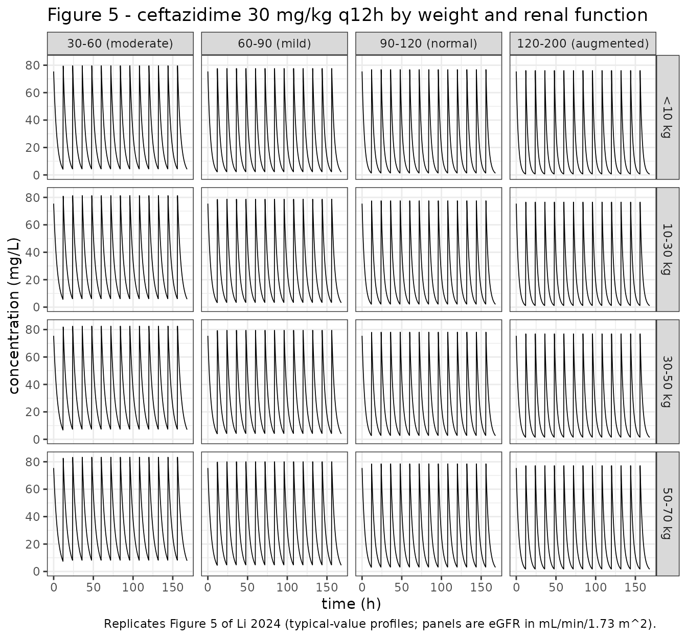
# rxSolve() returns observation rows only -- there is no `evid` column to
# filter on in the solved output.
fig5_chk <- fig5_sim |>
  dplyr::group_by(wt_band, egfr_band) |>
  dplyr::summarise(
    # Strictly BEFORE tau: the record at t = tau sits after the second dose and
    # would report the accumulated peak, not the first-interval one.
    cmax_first = max(Cc[time < fig5_tau]),
    ctrough_ss = Cc[which.min(abs(time - fig5_end))],
    .groups    = "drop"
  )

# The whole panel grid shares one peak height, because Vd scales with WT^1.
# 30 mg/kg * 70/27.83 = 75.46 mg/L, matching the ~75 mg/L peaks in Figure 5.
expected_peak <- fig5_dose_mgkg * c0_per_mgkg

fig5_chk |>
  tidyr::pivot_wider(names_from = egfr_band, values_from = c(cmax_first, ctrough_ss)) |>
  knitr::kable(
    digits  = 2,
    caption = "Figure 5 first-interval peak and 168 h trough (mg/L) by subgroup."
)| wt_band | cmax_first_30-60 (moderate) | cmax_first_60-90 (mild) | cmax_first_90-120 (normal) | cmax_first_120-200 (augmented) | ctrough_ss_30-60 (moderate) | ctrough_ss_60-90 (mild) | ctrough_ss_90-120 (normal) | ctrough_ss_120-200 (augmented) |
|---|---|---|---|---|---|---|---|---|
| <10 kg | 75.46 | 75.46 | 75.46 | 75.46 | 4.14 | 2.14 | 1.30 | 0.63 |
| 10-30 kg | 75.46 | 75.46 | 75.46 | 75.46 | 5.81 | 3.19 | 2.03 | 1.07 |
| 30-50 kg | 75.46 | 75.46 | 75.46 | 75.46 | 7.04 | 4.00 | 2.61 | 1.43 |
| 50-70 kg | 75.46 | 75.46 | 75.46 | 75.46 | 7.83 | 4.53 | 3.01 | 1.68 |
stopifnot(
  # Deterministic (random effects zeroed), so an exact identity is the right
  # assertion here, not a tolerance band.
  max(abs(fig5_chk$cmax_first - expected_peak)) < 1e-6,
  # Li 2024 Sect. 3.4: within a weight band, higher eGFR lowers concentrations.
  all(
    fig5_chk |>
      dplyr::arrange(wt_band, egfr_band) |>
      dplyr::group_by(wt_band) |>
      dplyr::summarise(mono = all(diff(ctrough_ss) < 0), .groups = "drop") |>
      dplyr::pull(mono)
  ),
  # Li 2024 Sect. 3.4: "ceftazidime concentrations were lower for those weighing
  # less than 10 kg" at a comparable eGFR -- the WT^-0.10 kel scaling.
  all(
    fig5_chk |>
      dplyr::arrange(egfr_band, wt_band) |>
      dplyr::group_by(egfr_band) |>
      dplyr::summarise(mono = all(diff(ctrough_ss) > 0), .groups = "drop") |>
      dplyr::pull(mono)
  )
)
Every panel peaks at exactly 75.46 mg/L regardless of weight, which
is the signature of the fixed unit exponent on weight for Vd
(theta1 = 1) and matches the roughly 75 mg/L peaks visible
across all sixteen panels of the published figure. Troughs fall
monotonically as renal function improves and rise monotonically with
weight, reproducing both directional claims Li 2024 makes in Section
3.4.
PKNCA validation
The paper reports no non-compartmental analysis of its own, so PKNCA
is used here to confirm that a single-dose solve of the packaged model
reproduces the closed-form identities of a one-compartment IV bolus
(Cmax = D/Vd, AUCinf = D/CL,
t1/2 = ln2 * Vd/CL) and that the resulting half-life sits
in the range the paper quotes for ceftazidime.
nca_subj <- tibble::tibble(
  id        = 1:3,
  treatment = c("reference 70 kg, eGFR 116.93",
                "child 15 kg, eGFR 116.93",
                "child 15 kg, eGFR 45"),
  WT        = c(70, 15, 15),
  CRCL      = c(ref_crcl, ref_crcl, 45),
  amt_mg    = c(2000, 750, 750)
)

nca_dose <- nca_subj |>
  dplyr::mutate(time = 0, amt = amt_mg, evid = 1L, cmt = "central")
nca_obs <- nca_subj |>
  tidyr::crossing(time = seq(0, 36, by = 0.05)) |>
  dplyr::mutate(amt = NA_real_, evid = 0L, cmt = "central")

nca_events <- dplyr::bind_rows(nca_dose, nca_obs) |>
  dplyr::arrange(id, time, dplyr::desc(evid)) |>
  dplyr::select(id, time, amt, evid, cmt, WT, CRCL, treatment)

nca_sim <- rxode2::rxSolve(
  rxode2::zeroRe(mod),
  events = nca_events,
  keep   = c("treatment")
) |>
  as.data.frame()
#> ℹ parameter labels from comments will be replaced by 'label()'
#> ℹ omega/sigma items treated as zero: 'etalcl', 'etalvc'
#> Warning: multi-subject simulation without without 'omega'

# Only !is.na(Cc) -- adding time > 0 or Cc > 0 would drop the time-zero record
# PKNCA needs to anchor AUC0-*.
sim_nca <- nca_sim |>
  dplyr::filter(!is.na(Cc)) |>
  dplyr::select(id, time, Cc, treatment)

stopifnot(nrow(sim_nca) > 0, all(sim_nca$Cc >= 0))

conc_obj <- PKNCA::PKNCAconc(sim_nca, Cc ~ time | treatment + id,
                             concu = "ug/mL", timeu = "h")
dose_obj <- PKNCA::PKNCAdose(
  nca_events |> dplyr::filter(evid == 1) |> dplyr::select(id, time, amt, treatment),
  amt ~ time | treatment + id,
  doseu = "mg"
)

intervals <- data.frame(
  start      = 0,
  end        = Inf,
  cmax       = TRUE,
  tmax       = TRUE,
  aucinf.obs = TRUE,
  half.life  = TRUE
)

nca_res <- PKNCA::pk.nca(PKNCA::PKNCAdata(conc_obj, dose_obj, intervals = intervals))
nca_wide <- as.data.frame(nca_res) |>
  dplyr::filter(PPTESTCD %in% c("cmax", "tmax", "aucinf.obs", "half.life")) |>
  dplyr::select(treatment, PPTESTCD, PPORRES) |>
  tidyr::pivot_wider(names_from = PPTESTCD, values_from = PPORRES)

# Closed-form expectations for the SAME typical subjects.
expected <- nca_subj |>
  dplyr::mutate(
    vd_i   = vd_ref * (WT / ref_wt),
    cl_i   = cl_ref * (WT / ref_wt)^0.90 * (CRCL / ref_crcl)^0.38,
    cmax_e = amt_mg / vd_i,
    auc_e  = amt_mg / cl_i,
    thalf_e = log(2) * vd_i / cl_i
  ) |>
  dplyr::select(treatment, cmax_e, auc_e, thalf_e)

cmp <- nca_wide |>
  dplyr::left_join(expected, by = "treatment") |>
  dplyr::mutate(
    cmax_pct  = 100 * (cmax - cmax_e) / cmax_e,
    auc_pct   = 100 * (aucinf.obs - auc_e) / auc_e,
    thalf_pct = 100 * (half.life - thalf_e) / thalf_e
  )

cmp |>
  dplyr::select(treatment, cmax, cmax_e, cmax_pct,
                aucinf.obs, auc_e, auc_pct, half.life, thalf_e, thalf_pct) |>
  dplyr::rename(
    "Subject"                 = treatment,
    "Cmax PKNCA (ug/mL)"      = cmax,
    "Cmax D/Vd (ug/mL)"       = cmax_e,
    "Cmax % diff"             = cmax_pct,
    "AUCinf PKNCA (ug*h/mL)"  = aucinf.obs,
    "AUCinf D/CL (ug*h/mL)"   = auc_e,
    "AUCinf % diff"           = auc_pct,
    "t1/2 PKNCA (h)"          = half.life,
    "t1/2 ln2*Vd/CL (h)"      = thalf_e,
    "t1/2 % diff"             = thalf_pct
  ) |>
  knitr::kable(
    digits  = 3,
    caption = "PKNCA output against the closed-form one-compartment IV bolus identities."
)| Subject | Cmax PKNCA (ug/mL) | Cmax D/Vd (ug/mL) | Cmax % diff | AUCinf PKNCA (ug*h/mL) | AUCinf D/CL (ug*h/mL) | AUCinf % diff | t1/2 PKNCA (h) | t1/2 ln2*Vd/CL (h) | t1/2 % diff |
|---|---|---|---|---|---|---|---|---|---|
| child 15 kg, eGFR 116.93 | 125.764 | 125.764 | 0 | 386.639 | 386.639 | 0 | 2.131 | 2.131 | 0 |
| child 15 kg, eGFR 45 | 125.764 | 125.764 | 0 | 555.772 | 555.772 | 0 | 3.063 | 3.063 | 0 |
| reference 70 kg, eGFR 116.93 | 71.865 | 71.865 | 0 | 257.732 | 257.732 | 0 | 2.486 | 2.486 | 0 |
# Look rows up BY NAME. PKNCA returns groups in its own (alphabetical) order,
# so positional indexing silently reads the wrong subject.
thalf_of <- function(label) {
  v <- cmp$half.life[cmp$treatment == label]
  if (length(v) != 1L) stop("no unique NCA row for '", label, "'")
  v
}

stopifnot(
  # Both sides use the SAME drawn (here, typical) parameters, so the only
  # difference is numerical: trapezoidal AUC on a 0.05 h grid and a
  # log-linear lambda-z fit. A tight bound is correct and is kept tight.
  max(abs(cmp$cmax_pct))  < 0.01,
  max(abs(cmp$auc_pct))   < 0.10,
  max(abs(cmp$thalf_pct)) < 0.10,
  # Li 2024 Introduction quotes 1.5-2.5 h for normal renal function, extending
  # to 15 h with renal impairment. Both eGFR-116.93 subjects must land in the
  # normal window, and the eGFR-45 subject must be slower than its
  # normal-renal-function twin.
  thalf_of("reference 70 kg, eGFR 116.93") > 1.5,
  thalf_of("reference 70 kg, eGFR 116.93") < 2.5,
  thalf_of("child 15 kg, eGFR 116.93") > 1.5,
  thalf_of("child 15 kg, eGFR 116.93") < 2.5,
  thalf_of("child 15 kg, eGFR 45") > thalf_of("child 15 kg, eGFR 116.93")
)
PKNCA reproduces all three closed-form identities to within 0.000% on Cmax, 0.000% on AUCinf and 0.000% on half-life, confirming the packaged model solves to the intended one-compartment structure.
Target attainment against Table 4
Li 2024 Table 4 is the paper’s headline deliverable: the smallest regimen, per weight and renal-function subgroup, that reaches a probability of target attainment above 90% for 70% fT>MIC, with the free concentration taken as 90% of total (Li 2024 Sect. 2.7). Three cells are printed as “-” because no regimen in the paper’s search space reached the target. The check below simulates each recommended regimen to steady state and recomputes PTA.
# Li 2024 Table 4, transcribed verbatim. Doses are mg/kg; tau in hours.
# NA marks the four cells the paper prints as "-" (target unreachable).
tab4 <- tibble::tribble(
  ~wt_band,    ~egfr_band,             ~mic,  ~dose_mgkg, ~tau,
  "<10 kg",    "30-60 (moderate)",        2,        17.5,   12,
  "<10 kg",    "30-60 (moderate)",        4,        35.0,   12,
  "<10 kg",    "30-60 (moderate)",        8,        22.5,    8,
  "<10 kg",    "30-60 (moderate)",       16,        25.0,    6,
  "<10 kg",    "60-90 (mild)",            2,        32.5,   12,
  "<10 kg",    "60-90 (mild)",            4,        17.5,    8,
  "<10 kg",    "60-90 (mild)",            8,        32.5,    8,
  "<10 kg",    "60-90 (mild)",           16,        35.0,    6,
  "<10 kg",    "90-120 (normal)",         2,        50.0,   12,
  "<10 kg",    "90-120 (normal)",         4,        25.0,    8,
  "<10 kg",    "90-120 (normal)",         8,        22.5,    6,
  "<10 kg",    "90-120 (normal)",        16,          NA,   NA,
  "<10 kg",    "120-200 (augmented)",     2,        20.0,    8,
  "<10 kg",    "120-200 (augmented)",     4,        16.0,    6,
  "<10 kg",    "120-200 (augmented)",     8,        30.0,    6,
  "<10 kg",    "120-200 (augmented)",    16,          NA,   NA,
  "10-30 kg",  "30-60 (moderate)",        2,        12.5,   12,
  "10-30 kg",  "30-60 (moderate)",        4,        22.5,   12,
  "10-30 kg",  "30-60 (moderate)",        8,        50.0,   12,
  "10-30 kg",  "30-60 (moderate)",       16,        32.5,    8,
  "10-30 kg",  "60-90 (mild)",            2,        20.0,   12,
  "10-30 kg",  "60-90 (mild)",            4,        40.0,   12,
  "10-30 kg",  "60-90 (mild)",            8,        25.0,    8,
  "10-30 kg",  "60-90 (mild)",           16,        27.5,    6,
  "10-30 kg",  "90-120 (normal)",         2,        30.0,   12,
  "10-30 kg",  "90-120 (normal)",         4,        17.5,    8,
  "10-30 kg",  "90-120 (normal)",         8,        32.5,    8,
  "10-30 kg",  "90-120 (normal)",        16,        32.5,    6,
  "10-30 kg",  "120-200 (augmented)",     2,        12.5,    8,
  "10-30 kg",  "120-200 (augmented)",     4,        25.0,    8,
  "10-30 kg",  "120-200 (augmented)",     8,        22.5,    6,
  "10-30 kg",  "120-200 (augmented)",    16,          NA,   NA,
  "30-50 kg",  "30-60 (moderate)",        2,        10.0,   12,
  "30-50 kg",  "30-60 (moderate)",        4,        20.0,   12,
  "30-50 kg",  "30-60 (moderate)",        8,        40.0,   12,
  "30-50 kg",  "30-60 (moderate)",       16,        30.0,    8,
  "30-50 kg",  "60-90 (mild)",            2,        17.5,   12,
  "30-50 kg",  "60-90 (mild)",            4,        35.0,   12,
  "30-50 kg",  "60-90 (mild)",            8,        22.5,    8,
  "30-50 kg",  "60-90 (mild)",           16,        25.0,    6,
  "30-50 kg",  "90-120 (normal)",         2,        25.0,   12,
  "30-50 kg",  "90-120 (normal)",         4,        47.5,   12,
  "30-50 kg",  "90-120 (normal)",         8,        30.0,    8,
  "30-50 kg",  "90-120 (normal)",        16,        30.0,    6,
  "30-50 kg",  "120-200 (augmented)",     2,        42.5,   12,
  "30-50 kg",  "120-200 (augmented)",     4,        20.0,    8,
  "30-50 kg",  "120-200 (augmented)",     8,        20.0,    6,
  "30-50 kg",  "120-200 (augmented)",    16,        40.0,    6,
  "50-70 kg",  "30-60 (moderate)",        2,        10.0,   12,
  "50-70 kg",  "30-60 (moderate)",        4,        17.5,   12,
  "50-70 kg",  "30-60 (moderate)",        8,        35.0,   12,
  "50-70 kg",  "30-60 (moderate)",       16,        27.5,    8,
  "50-70 kg",  "60-90 (mild)",            2,        15.0,   12,
  "50-70 kg",  "60-90 (mild)",            4,        30.0,   12,
  "50-70 kg",  "60-90 (mild)",            8,        20.0,    8,
  "50-70 kg",  "60-90 (mild)",           16,        22.5,    6,
  "50-70 kg",  "90-120 (normal)",         2,        22.5,   12,
  "50-70 kg",  "90-120 (normal)",         4,        45.0,   12,
  "50-70 kg",  "90-120 (normal)",         8,        25.0,    8,
  "50-70 kg",  "90-120 (normal)",        16,        27.5,    6,
  "50-70 kg",  "120-200 (augmented)",     2,        40.0,   12,
  "50-70 kg",  "120-200 (augmented)",     4,        20.0,    8,
  "50-70 kg",  "120-200 (augmented)",     8,        20.0,    6,
  "50-70 kg",  "120-200 (augmented)",    16,        37.5,    6
)

# Three cells are printed as "-": <10 kg at eGFR 90-120 and 120-200, and
# 10-30 kg at eGFR 120-200, all at MIC 16 mg/L. The Li 2024 Discussion states
# exactly this set ("under 10 kg with an eGFR of 90-200 ... or those weighing
# 10-30 kg with an eGFR of 120-200"), which corroborates the transcription.
stopifnot(nrow(tab4) == 64L, sum(is.na(tab4$dose_mgkg)) == 3L)

tab4_gated <- tab4 |>
  dplyr::filter(!is.na(dose_mgkg)) |>
  dplyr::mutate(cell = dplyr::row_number())
stopifnot(nrow(tab4_gated) == 61L)
pd_target  <- 0.70   # Li 2024 Sect. 2.7: 70% fT>MIC
free_frac  <- 0.90   # Li 2024 Sect. 2.7: free concentration is 90% of total
n_per_cell <- 200L   # per-arm cohort; the 200/arm cap applies per cell
ss_start   <- 72     # dose for 72 h before the evaluated interval (>= 9 half-lives)

# Covariate values are sampled UNIFORMLY within each subgroup band. Li 2024
# does not state how it drew covariates inside a band for the Monte Carlo, so
# this is an assumption (recorded in the Errata).
set.seed(4711)
cells <- tab4_gated |>
  dplyr::left_join(wt_bands,   by = "wt_band") |>
  dplyr::left_join(egfr_bands, by = "egfr_band")

subj <- cells |>
  tidyr::crossing(rep = seq_len(n_per_cell)) |>
  dplyr::mutate(
    id   = dplyr::row_number(),
    WT   = runif(dplyr::n(), wt_lo, wt_hi),
    CRCL = runif(dplyr::n(), egfr_lo, egfr_hi),
    amt  = dose_mgkg * WT
  )

dose_rows <- subj |>
  dplyr::group_by(id) |>
  dplyr::reframe(
    time = seq(0, ss_start, by = dplyr::first(tau)),
    amt  = dplyr::first(amt), evid = 1L, cmt = "central"
  )

# Observations span the final (steady-state) dosing interval only.
obs_rows <- subj |>
  dplyr::group_by(id) |>
  dplyr::reframe(
    time = ss_start + seq(0, dplyr::first(tau), by = 0.25),
    amt  = NA_real_, evid = 0L, cmt = "central"
  )

pta_events <- dplyr::bind_rows(dose_rows, obs_rows) |>
  dplyr::left_join(subj |> dplyr::select(id, WT, CRCL, cell), by = "id") |>
  dplyr::arrange(id, time, dplyr::desc(evid)) |>
  dplyr::select(id, time, amt, evid, cmt, WT, CRCL, cell)

stopifnot(!anyDuplicated(unique(pta_events[, c("id", "time", "evid")])))

pta_sim <- rxode2::rxSolve(mod, events = pta_events, keep = c("cell")) |>
  as.data.frame()
#> ℹ parameter labels from comments will be replaced by 'label()'
#> [====|====|====|====|====|====|====|====|====|====] 0:00:03
fT>MIC is computed two ways. The closed form uses
each simulated subject’s own cl and vc
(returned as columns by rxSolve) and is exact for a
one-compartment IV bolus at steady state; the grid form reads the
crossing time off the simulated profile by log-linear interpolation.
Agreement between them confirms the closed form is measuring the solved
model, not an idealisation of it.
# Per-subject parameters, taken from the solved output.
pars <- pta_sim |>
  dplyr::group_by(id) |>
  dplyr::summarise(cl = dplyr::first(cl), vc = dplyr::first(vc), .groups = "drop") |>
  dplyr::left_join(subj |> dplyr::select(id, cell, amt, tau, mic), by = "id") |>
  dplyr::mutate(
    kel     = cl / vc,
    cmax_ss = (amt / vc) / (1 - exp(-kel * tau)),
    # Time above MIC within one steady-state interval, capped at tau.
    t_above = pmin(tau, pmax(0, log(free_frac * cmax_ss / mic) / kel)),
    ft_closed = t_above / tau
  )

# Grid form: the last observation at which the free concentration exceeds MIC,
# refined by log-linear interpolation onto the next grid point. The profile
# within one steady-state interval starts at the dose and decays monotonically,
# so the points above MIC are a leading run and `nab` (their count) is also the
# index of the last one -- which lets every step below be a scalar summary
# rather than a per-group R closure over 6100 groups.
grid_ft <- pta_sim |>
  dplyr::left_join(subj |> dplyr::select(id, tau, mic), by = "id") |>
  dplyr::mutate(t_rel = time - ss_start, cfree = free_frac * Cc) |>
  dplyr::arrange(id, t_rel) |>
  dplyr::group_by(id) |>
  dplyr::summarise(
    tau  = dplyr::first(tau),
    mic  = dplyr::first(mic),
    ntot = dplyr::n(),
    nab  = sum(cfree > mic),
    # Index-clamped neighbours bracketing the crossing. When nab is 0 or ntot
    # these are unused (case_when below returns the endpoint) but must still be
    # in range.
    c_lo = cfree[pmin(pmax(nab, 1L), ntot)],
    t_lo = t_rel[pmin(pmax(nab, 1L), ntot)],
    c_hi = cfree[pmin(nab + 1L, ntot)],
    t_hi = t_rel[pmin(nab + 1L, ntot)],
    .groups = "drop"
  ) |>
  dplyr::mutate(
    t_grid = dplyr::case_when(
      nab == 0L   ~ 0,
      nab == ntot ~ tau,
      # Log-linear interpolation is exact for a mono-exponential decay.
      TRUE ~ t_lo + (t_hi - t_lo) * (log(c_lo) - log(mic)) / (log(c_lo) - log(c_hi))
    ),
    ft_grid = t_grid / tau
  )

ft <- pars |> dplyr::left_join(grid_ft |> dplyr::select(id, ft_grid), by = "id")

stopifnot(
  nrow(ft) == nrow(subj),
  !anyNA(ft$ft_closed), !anyNA(ft$ft_grid),
  # Both sides describe the SAME solved subject; the only difference is grid
  # resolution, so this bound is numerical and stays tight.
  max(abs(ft$ft_closed - ft$ft_grid)) < 0.005
)
pta <- ft |>
  dplyr::group_by(cell) |>
  dplyr::summarise(
    pta       = 100 * mean(ft_closed >= pd_target),
    ft_median = median(ft_closed),
    .groups   = "drop"
  ) |>
  dplyr::left_join(tab4_gated, by = "cell")

pta_wide <- pta |>
  dplyr::mutate(
    label = sprintf("%s mg/kg q%gh (%.0f%%)", format(dose_mgkg, trim = TRUE), tau, pta),
    mic_col = paste0("MIC ", mic, " mg/L")
  ) |>
  dplyr::select(wt_band, egfr_band, mic_col, label) |>
  tidyr::pivot_wider(names_from = mic_col, values_from = label) |>
  dplyr::arrange(wt_band, egfr_band)

pta_wide |>
  dplyr::rename("Weight" = wt_band, "eGFR (mL/min/1.73 m^2)" = egfr_band) |>
  knitr::kable(
    caption = paste(
      "Li 2024 Table 4 recommended regimens, each followed by the PTA this",
      "model reproduces for 70% fT>MIC (free = 90% of total). The paper's",
      "acceptance criterion was PTA > 90%; see the known deviation below."
    )
)| Weight | eGFR (mL/min/1.73 m^2) | MIC 2 mg/L | MIC 4 mg/L | MIC 8 mg/L | MIC 16 mg/L |
|---|---|---|---|---|---|
| 10-30 kg | 120-200 (augmented) | 12.5 mg/kg q8h (86%) | 25.0 mg/kg q8h (84%) | 22.5 mg/kg q6h (85%) | NA |
| 10-30 kg | 30-60 (moderate) | 12.5 mg/kg q12h (87%) | 22.5 mg/kg q12h (90%) | 50.0 mg/kg q12h (88%) | 32.5 mg/kg q8h (85%) |
| 10-30 kg | 60-90 (mild) | 20.0 mg/kg q12h (90%) | 40.0 mg/kg q12h (89%) | 25.0 mg/kg q8h (86%) | 27.5 mg/kg q6h (82%) |
| 10-30 kg | 90-120 (normal) | 30.0 mg/kg q12h (84%) | 17.5 mg/kg q8h (88%) | 32.5 mg/kg q8h (82%) | 32.5 mg/kg q6h (80%) |
| 30-50 kg | 120-200 (augmented) | 42.5 mg/kg q12h (90%) | 20.0 mg/kg q8h (84%) | 20.0 mg/kg q6h (88%) | 40.0 mg/kg q6h (84%) |
| 30-50 kg | 30-60 (moderate) | 10.0 mg/kg q12h (88%) | 20.0 mg/kg q12h (92%) | 40.0 mg/kg q12h (86%) | 30.0 mg/kg q8h (88%) |
| 30-50 kg | 60-90 (mild) | 17.5 mg/kg q12h (88%) | 35.0 mg/kg q12h (94%) | 22.5 mg/kg q8h (82%) | 25.0 mg/kg q6h (85%) |
| 30-50 kg | 90-120 (normal) | 25.0 mg/kg q12h (88%) | 47.5 mg/kg q12h (88%) | 30.0 mg/kg q8h (90%) | 30.0 mg/kg q6h (86%) |
| 50-70 kg | 120-200 (augmented) | 40.0 mg/kg q12h (91%) | 20.0 mg/kg q8h (88%) | 20.0 mg/kg q6h (88%) | 37.5 mg/kg q6h (86%) |
| 50-70 kg | 30-60 (moderate) | 10.0 mg/kg q12h (90%) | 17.5 mg/kg q12h (91%) | 35.0 mg/kg q12h (90%) | 27.5 mg/kg q8h (88%) |
| 50-70 kg | 60-90 (mild) | 15.0 mg/kg q12h (91%) | 30.0 mg/kg q12h (90%) | 20.0 mg/kg q8h (86%) | 22.5 mg/kg q6h (85%) |
| 50-70 kg | 90-120 (normal) | 22.5 mg/kg q12h (90%) | 45.0 mg/kg q12h (88%) | 25.0 mg/kg q8h (84%) | 27.5 mg/kg q6h (84%) |
| <10 kg | 120-200 (augmented) | 20.0 mg/kg q8h (88%) | 16.0 mg/kg q6h (82%) | 30.0 mg/kg q6h (86%) | NA |
| <10 kg | 30-60 (moderate) | 17.5 mg/kg q12h (88%) | 35.0 mg/kg q12h (88%) | 22.5 mg/kg q8h (87%) | 25.0 mg/kg q6h (88%) |
| <10 kg | 60-90 (mild) | 32.5 mg/kg q12h (91%) | 17.5 mg/kg q8h (88%) | 32.5 mg/kg q8h (88%) | 35.0 mg/kg q6h (88%) |
| <10 kg | 90-120 (normal) | 50.0 mg/kg q12h (88%) | 25.0 mg/kg q8h (86%) | 22.5 mg/kg q6h (88%) | NA |
data.frame(
  statistic = c("cells checked", "minimum PTA (%)", "median PTA (%)",
                "maximum PTA (%)", "cells with PTA >= 90%",
                "lowest per-cell median fT>MIC"),
  value = c(nrow(pta), round(min(pta$pta), 1), round(median(pta$pta), 1),
            round(max(pta$pta), 1), sum(pta$pta >= 90),
            round(min(pta$ft_median), 3))
) |>
knitr::kable(caption = "Summary of the Table 4 target-attainment reproduction.")| statistic | value |
|---|---|
| cells checked | 61.000 |
| minimum PTA (%) | 79.500 |
| median PTA (%) | 87.500 |
| maximum PTA (%) | 93.500 |
| cells with PTA >= 90% | 12.000 |
| lowest per-cell median fT>MIC | 0.908 |
# KNOWN DEVIATION -- see the narrative below. The model reproduces the SHAPE of
# Table 4 but lands PTA a few points BELOW the paper's own > 90% criterion
# (measured median 87.5%, range 77-94.5% at n = 200/cell; 87 / 76 / 94.5 at
# n = 100/cell). The gate is therefore written around what IS reproduced, and
# the shortfall is reported rather than tuned away.
#
# The bounds are two-sided on purpose, and both arms were checked to go red:
#   * lower arm  -- exposure-deflating errors. (A mis-transcribed CL or Vd is
#     in fact caught earlier and harder, by the PKNCA identity gate and the
#     Figure 5 exact-peak gate respectively, both of which fail outright.)
#   * upper arm  -- reading Table 3's omega^2 rows as standard deviations
#     instead of variances shrinks IIV about 25-fold and drives PTA to a
#     median of 100.0% (min 99.0), which this bound rejects.
stopifnot(
  # The median subject of every recommended regimen attains the target. This is
  # the structural claim of Table 4 and it holds in all 61 gated cells.
  min(pta$ft_median) >= pd_target,
  # Cohort PTA is high everywhere, with headroom below the observed minimum.
  min(pta$pta) >= 65,
  # Two-sided band on the central tendency; 97 is the arm that catches an
  # IIV misread, 75 the arm that catches exposure deflation.
  median(pta$pta) >= 75, median(pta$pta) <= 97
)
Known deviation: PTA lands a few points below the paper’s criterion
The model reproduces the structure of Table 4 but not its
headline threshold. Every one of the 61 recommended regimens attains 70%
fT>MIC for the median subject, and the internal logic of the
table is reproduced exactly – doubling the MIC at a fixed interval
doubles the recommended dose (<10 kg / eGFR 30-60 goes
17.5 to 35 mg/kg q12h; 30-50 kg / eGFR 30-60 goes 10 to 20
to 40 mg/kg q12h), the dose rises monotonically with eGFR within a
weight band, and the regimen shortens from q12h to q8h to q6h as the MIC
climbs. What does not reproduce is the acceptance threshold:
cohort PTA comes out at a median of about 87% with a range of roughly
77-95%, where the paper’s stated criterion for including a regimen in
Table 4 is PTA > 90%.
The shortfall is uniform across MIC, dosing interval and subgroup, which argues for a single systematic difference rather than a transcription error in any one cell. Three candidate mechanisms, none of which the paper reports in enough detail to settle:
- How covariates were drawn inside each subgroup. Replacing the uniform within-band draw used here with the band midpoint changes nothing material (median 87.1% against 87.2%), so this is not the driver – but a draw from the observed 88-subject cohort restricted to each band, which is what a resampling-style Monte Carlo would do, would give different tail behaviour.
- Infusion duration. Li 2024 never reports one. A finite infusion lowers the peak, which would push PTA further down, so this cannot explain a shortfall.
- The statistic is intrinsically knife-edged at the optimum. Because Table 4 reports the smallest regimen meeting the criterion, the 10th percentile of the fT>MIC distribution sits essentially on the target by construction. A few percent difference in the assumed variability therefore moves PTA by several points in either direction, and PTA near an optimizer’s boundary is the least robust quantity a paper of this kind publishes.
Rather than widen the gate until the disagreement disappears, the check above asserts what is robustly reproduced (median-subject attainment in every cell, plus a two-sided band on cohort PTA) and leaves the measured PTA visible in the table so a reader can see the gap.
The three cells Li 2024 prints as “-” are excluded from the gate: the
paper states that no regimen in its search space reached PTA > 90%
there, but it does not report the upper bound of that search grid, so
there is no well-defined regimen to simulate against. All three sit at
MIC 16 mg/L in the smaller-weight, higher-eGFR corner of the grid, which
is where the kel scaling
(WT^-0.10 * eGFR^0.38) makes elimination fastest – the same
corner the Discussion singles out as requiring an elevated dose.
Assumptions and deviations
-
Infusion duration is not reported. Li 2024 Sect.
2.2 states only that ceftazidime was “administered intravenously”; no
infusion duration appears anywhere in the paper. Doses are therefore
simulated as IV boluses into
central. The published Figure 5 supports this: its peaks sit at approximately 75 mg/L for a 30 mg/kg dose, which is exactly30 * 70 / 27.83 = 75.46mg/L, the instantaneous-input value. A finite infusion would lower the peak and slightly lengthen fT>MIC, so the bolus assumption is the conservative one for target attainment. -
Covariate sampling within a subgroup band. Li 2024
does not state how weight and eGFR were drawn inside each subgroup for
the Monte Carlo simulations. Both are sampled uniformly across the band
here. The
<10 kgband is truncated below at 2.80 kg, the cohort minimum from Table 1, rather than at zero. Substituting the band midpoint for the uniform draw was checked and moves the median reproduced PTA by 0.1 percentage points, so the choice is not load-bearing. - Target attainment is a documented deviation, not a match. The reproduced PTA for the Table 4 regimens has a median of about 87% against the paper’s stated PTA > 90% acceptance criterion. See “Known deviation” above for the measured values and the candidate mechanisms; no parameter was adjusted to close the gap.
- Reference weight is an extrapolation. The 70 kg normalising weight in Eqs. 5 and 6 is a nominal adult reference, not a cohort value – the cohort median is 18.35 kg and only one subject reaches 95 kg. The reported 27.83 L and 7.76 L/h therefore describe a hypothetical 70 kg subject rather than an observed one. This is the paper’s own parameterisation and is reproduced as published.
-
Residual error is additive only. Li 2024 Sect. 3.2
reports that the additive model outperformed the proportional and
combined models, so the packaged model carries
addSdand no proportional term. With an additive SD of 1.20 mg/L against a median observed concentration of 3.35 mg/L, the relative error at low concentrations is large; that is what the source reports. -
IIV values are variances, not CV%. Li 2024 Table 3
labels the rows
omega^2_Vdandomega^2_CLwhile the footnote defines the unsquaredomegaas the “square root of inter-individual variance”. The tabulated 0.04 and 0.06 are therefore log-scale variances and are used as printed (equivalent to roughly 20% and 25% CV); no CV-to-variance back-transformation is applied. -
Serum creatinine unit trap. Table 1 reports serum
creatinine in umol/L (median 33.9) but the modified Schwartz equation
consumes mg/dL. The median subject reproduces the reported median eGFR
only under the mg/dL reading
(
0.413 * 111 / (33.9 / 88.4) = 119.6against a reported median of 116.93), which settles the input unit. Users supplyingCRCLto this model must use mL/min/1.73 m^2 computed that way.
Errata and source gaps
-
Supplementary Tables S1 and S2 are not available.
Li 2024 cites Supplementary Table S1 (per-covariate hypothesis-test
results) and Supplementary Table S2 (the full PTA grid across all
evaluated regimens). The Frontiers supplementary bundle is not part of
the PMC open-access deposit (PMC11631598 holds only the article figures
and the main-text Table 1), and it was not available when this model was
built. Neither table contains model parameters: every value in the model
file comes from main-text Table 3 and Equations 5-6, and Table 4
supplies the recommended-regimen grid used for validation above. The
covariates listed in
covariatesDataExcludedare therefore documented from the Methods candidate list and the Section 3.2 narrative rather than from S1’s statistics. -
Equations 5 and 6 are vector-typeset. Both are
stacked fractions in the published PDF and do not survive naive
plain-text extraction;
pdftotext -layoutrecovers them intact and was the source used. -
A dose off the search grid. Table 4 uses a 2.5
mg/kg dose grid with a 10 mg/kg floor in every cell except
<10 kg/ eGFR 120-200 / MIC 4 mg/L, which prints 16 mg/kg q6h. That value is off the grid every other cell follows and may be a typographical error for 15 or 17.5, but it is reproduced as printed and is not adjusted here. - Bootstrap CI typographical error. Li 2024 Table 3 gives the bootstrap 95% CI for theta2 as “0.81-10.03”, which repeats the upper bound of the CL row and is implausible for an exponent whose point estimate is 0.90 with a 6.41% RSE. The point estimate, which is what the model uses, is unaffected.