Imatinib: fifteen published population PK models (Yang 2025 external evaluation)

library(nlmixr2lib)
library(rxode2)
library(PKNCA)
library(dplyr)
library(ggplot2)

Provenance: this is a transcription from a secondary source

Read this section before using any model on this page.

Yang and colleagues (2025) did not develop a population PK model. They performed a systematic review that identified fifteen previously published population PK models of imatinib, and then evaluated all fifteen against a real-world therapeutic-drug-monitoring (TDM) dataset of 39 adult and pediatric patients treated at Nordic centres. Their conclusion is negative and is stated in the title: the published models perform poorly, especially in children.

The standing policy for a secondary source is to skip it and extract the cited primary papers instead. The carve-out that applies here is that Yang 2025 Table 1 tabulates the parameters of every one of the fifteen models to an unusually complete standard: structural model, typical values, covariate coefficients with their centring constants, between-subject variability, and residual-error magnitudes, with table footnotes that resolve every categorical coefficient. Fourteen of those fifteen models are therefore transcribed into this package; the fifteenth, Jiang 2023, was already in the library, extracted directly from its primary publication.

Consequences you must keep in mind:

• Every parameter value in these fourteen files comes from Yang 2025 Table 1, not from the paper named in each file’s reference field. Each file says so in its description and repeats the citation chain in reference.
• Each file should be re-extracted from its primary when that paper is obtained. A review reprints values but routinely drops the host table’s footnotes, its model-selection rationale, and any structure the summary row only gestures at.
• Yang 2025 also evaluated an allometrically scaled variant of most models, in which standard allometry replaced the published weight terms. Those variants are Yang 2025’s own modification and are not encoded here. Each file is the model as published.
• Demographic detail beyond what Table 1 prints (weight ranges, sex splits, race) is unavailable from the secondary source and is recorded as such in each file’s population metadata.

The one model whose transcription can be checked directly is Jiang 2023, because the library already holds an independent extraction from its primary. Yang 2025 Table 1 gives CL/F = 9.72 x (RBC/3.7)^0.49 x theta_ABCG2 with theta = 0.879 (GT) and 0.976 (TT), Vc/F = 229 L, ka = 1.22 /h, CV%(CL) 13.9% and a 29.6% proportional residual. Jiang_2023_imatinib.R, extracted from Jiang 2023 itself, carries exactly those ten numbers. That is a clean ten-of-ten fidelity check on the secondary source’s transcription, and it is why the carve-out was applied.

The variability scale, and how it was settled

The single most dangerous ambiguity when transcribing a variance column out of a review is its scale: a number like 0.305 may be a variance, a standard deviation, or a coefficient of variation, and guessing wrong is a two-fold error in omega. Yang 2025 does better than most secondary sources here, because it labels each row with the scale it reports: Var(eta_CL) for Judson, omega_CL for Yamakawa, CV%(CL) for the remaining rows, and rho_CL-Vc for Gotta. Two rows nonetheless settle the question mechanically rather than by trusting the label, because each reports a covariance alongside its variability terms and a covariance constrains the implied correlation to lie in [-1, 1]:

• Judson 2005 reports Var(eta_CL) = 0.305, Var(eta_Vc) = 0.34, Cov = 0.237. Read as variances, the correlation is 0.237 / sqrt(0.305 x 0.34) = 0.736, which is admissible. Read as standard deviations, it is 0.237 / sqrt(0.093 x 0.116) = 2.29, which is impossible. The label Var is therefore correct.
• Demetri 2009 reports CV%(CL) = 34.6%, CV%(Vc) = 35.7%, Cov = 0.119. Taking omega = CV gives a correlation of 0.119 / (0.346 x 0.357) = 0.963, admissible. Taking the exact log-normal conversion omega^2 = log(1 + CV^2) gives 0.119 / sqrt(0.1128 x 0.1198) = 1.024 > 1, impossible. So the CV% entries are converted as omega = CV/100, not by the exact log-normal formula.

The second rule matches the convention already used by the independently extracted Jiang_2023_imatinib.R, whose primary prints the variance directly as exp(0.0192) next to a tabulated IIV of 0.139 (0.139^2 = 0.0193). Every CV% entry in these fourteen files is therefore converted as variance = (CV/100)^2, and every omega entry (Yamakawa only) as variance = omega^2.

Source trace

Every parameter in every file traces to a single cell of Yang 2025 Table 1 (pages 876-877 of the article, spanning two printed pages), or to one of that table’s lettered footnotes. The per-file ini() blocks carry a trailing comment on each line naming the cell; the table below records the structural claim per model.

model_specs <- tibble::tribble(
  ~stem,                        ~label,                 ~primary_year, ~country,        ~n_subj, ~n_obs, ~diagnosis,
  "Judson_2005_imatinib",       "Judson 2005",          2005L,         "Europe + USA",   43L,     517L,   "GIST / STS",
  "Schmidli_2005_imatinib",     "Schmidli 2005",        2005L,         "Multi-country", 371L,    1930L,   "CML",
  "Widmer_2006_imatinib",       "Widmer 2006",          2006L,         "Switzerland",    59L,     321L,   "GIST / CML / ALL",
  "Petain_2008_imatinib",       "Petain 2008",          2008L,         "France",         67L,     505L,   "Solid tumours / GIST",
  "Demetri_2009_imatinib",      "Demetri 2009",         2009L,         "Europe + USA",   73L,      NA,    "GIST",
  "MenonAndersen_2009_imatinib","Menon-Andersen 2009",  2009L,         "USA",            41L,     842L,   "Ph+ leukemia / solid tumour",
  "Yamakawa_2011_imatinib",     "Yamakawa 2011",        2011L,         "Japan",          34L,     622L,   "CML",
  "Eechoute_2012_imatinib",     "Eechoute 2012",        2012L,         "Europe",         50L,    1743L,   "GIST",
  "Golabchifar_2014_imatinib",  "Golabchifar 2014",     2014L,         "Iran",           61L,     533L,   "CML",
  "Gotta_2014_imatinib",        "Gotta 2014",           2014L,         "Europe",       2478L,    4095L,   "CML",
  "DiPaolo_2014_imatinib",      "Di Paolo 2014",        2014L,         "Italy",          60L,     117L,   "CML",
  "Wang_2019_imatinib",         "Wang 2019",            2019L,         "China",         170L,     229L,   "CML",
  "Shriyan_2022_imatinib",      "Shriyan 2022",         2022L,         "India",          49L,     221L,   "CML",
  "Jiang_2023_imatinib",        "Jiang 2023",           2023L,         "China",         110L,      NA,    "GIST",
  "He_2023_imatinib",           "He 2023",              2023L,         "China",         230L,     424L,   "CML"
)

stopifnot(nrow(model_specs) == 15L)
# readModelDb() returns the model-defining function; rxode() evaluates it into
# the rxUi object that carries $state, $theta, $allCovs and can be solved.
models <- lapply(model_specs$stem, function(s) rxode2::rxode(nlmixr2lib::readModelDb(s)))
#> ℹ parameter labels from comments will be replaced by 'label()'
#> ℹ parameter labels from comments will be replaced by 'label()'
#> ℹ parameter labels from comments will be replaced by 'label()'
#> ℹ parameter labels from comments will be replaced by 'label()'
#> ℹ parameter labels from comments will be replaced by 'label()'
#> ℹ parameter labels from comments will be replaced by 'label()'
#> ℹ parameter labels from comments will be replaced by 'label()'
#> ℹ parameter labels from comments will be replaced by 'label()'
#> ℹ parameter labels from comments will be replaced by 'label()'
#> ℹ parameter labels from comments will be replaced by 'label()'
#> ℹ parameter labels from comments will be replaced by 'label()'
#> ℹ parameter labels from comments will be replaced by 'label()'
#> ℹ parameter labels from comments will be replaced by 'label()'
#> ℹ parameter labels from comments will be replaced by 'label()'
#> ℹ parameter labels from comments will be replaced by 'label()'
names(models) <- model_specs$stem

Structural audit: an enumerating test against the paper’s own prose

Yang 2025 Results section 3.1 makes a series of arithmetic claims about the fifteen models it reviewed. Each is a count over the whole set, so each can be checked by enumerating the transcribed model files rather than by inspecting a few of them by hand. A claim that quantifies over every member of a set needs an enumerating test; hand-picked examples cannot fail in the right way.

The structural features below are derived from the model objects, not re-declared: the disposition compartment count from the presence of a peripheral1 state, zero-order absorption from a d1 term, a transit chain from transit* states, a lag time from a tlag term, and a metabolite sub-model from _ndmima-suffixed states.

describe_structure <- function(mod) {
  states <- mod$state
  thetas <- names(mod$theta)
  parent_states <- states[!grepl("_ndmima$", states)]
  tibble::tibble(
    n_disposition_cmt = 1L + sum(grepl("^peripheral[0-9]*$", parent_states)),
    zero_order        = "ld1" %in% thetas,
    transit_chain     = any(grepl("^transit[0-9]+$", states)),
    lag_time          = "ltlag" %in% thetas,
    metabolite        = any(grepl("_ndmima$", states)),
    covariates        = paste(sort(mod$allCovs), collapse = ", ")
  )
}

structure_tbl <-
  dplyr::bind_cols(
    model_specs[, c("label", "country", "n_subj")],
    dplyr::bind_rows(lapply(models, describe_structure))
  ) |>
  dplyr::mutate(
    absorption = dplyr::case_when(
      transit_chain ~ "transit (5 compartments)",
      zero_order & lag_time ~ "zero-order + lag",
      zero_order ~ "zero-order",
      TRUE ~ "first-order"
    )
  )

structure_tbl |>
  dplyr::select(label, country, n_subj, n_disposition_cmt, absorption, metabolite, covariates) |>
  dplyr::rename(
    "Model" = label,
    "Country / region" = country,
    "N subjects" = n_subj,
    "Disposition compartments" = n_disposition_cmt,
    "Absorption" = absorption,
    "Metabolite sub-model" = metabolite,
    "Covariates" = covariates
  ) |>
  knitr::kable(caption = "Structural summary of all fifteen transcribed models, derived from the model files. Replicates Table 1 of Yang 2025.")

Structural summary of all fifteen transcribed models, derived from the model files. Replicates Table 1 of Yang 2025.

Model	Country / region	N subjects	Disposition compartments	Absorption	Metabolite sub-model	Covariates
Judson 2005	Europe + USA	43	1	zero-order	FALSE	WT
Schmidli 2005	Multi-country	371	1	zero-order	FALSE	HGB, OCC, WBC, WT
Widmer 2006	Switzerland	59	1	first-order	FALSE
Petain 2008	France	67	1	first-order	TRUE	AAG, ALB, OCC, WT
Demetri 2009	Europe + USA	73	1	zero-order	FALSE	ALB, OCC, WBC
Menon-Andersen 2009	USA	41	1	zero-order	TRUE	WT
Yamakawa 2011	Japan	34	1	first-order	FALSE
Eechoute 2012	Europe	50	2	transit (5 compartments)	FALSE	T_FIRSTDOSE, TUM_VOL
Golabchifar 2014	Iran	61	1	zero-order + lag	FALSE
Gotta 2014	Europe	2478	1	zero-order	FALSE	AGE, SEXF
Di Paolo 2014	Italy	60	1	first-order	FALSE	AAG, SNP_SLC22A1_RS683369
Wang 2019	China	170	1	first-order	FALSE	WT
Shriyan 2022	India	49	1	zero-order	FALSE
Jiang 2023	China	110	1	first-order	FALSE	RBC, SNP_ABCG2_RS2231142_HET, SNP_ABCG2_RS2231142_HOM
He 2023	China	230	1	first-order	FALSE	CRCL, HGB

The counts Yang 2025 states in Results 3.1 are now assertions:

# "A one-compartment model was used in almost all the included models (N = 14),
#  except one that used a two-compartment model."
stopifnot(sum(structure_tbl$n_disposition_cmt == 1L) == 14L)
stopifnot(sum(structure_tbl$n_disposition_cmt == 2L) == 1L)

# "The absorption phase was characterized by first-order (N = 7), zero-order
#  (N = 7), and a transit model (N = 1)."
stopifnot(sum(structure_tbl$absorption == "first-order") == 7L)
stopifnot(sum(grepl("^zero-order", structure_tbl$absorption)) == 7L)
stopifnot(sum(structure_tbl$transit_chain) == 1L)

# "One study found a lag time in imatinib absorption."
stopifnot(sum(structure_tbl$lag_time) == 1L)

# "Two studies also included the PK profile of the main metabolite N-desmethyl
#  imatinib in their model."
stopifnot(sum(structure_tbl$metabolite) == 2L)

# "Total body weight was the most frequently identified covariate (N = 5).
#  Hemoglobin (N = 2), white blood cell count (N = 2), plasma AGP (N = 2), and
#  albumin (N = 2) were other covariates found more than once."
covariate_counts <- table(unlist(lapply(models, function(m) m$allCovs)))
stopifnot(covariate_counts[["WT"]] == 5L)
stopifnot(covariate_counts[["HGB"]] == 2L)
stopifnot(covariate_counts[["WBC"]] == 2L)
stopifnot(covariate_counts[["AAG"]] == 2L)
stopifnot(covariate_counts[["ALB"]] == 2L)

cat("All structural counts from Yang 2025 Results 3.1 reproduce.\n")
#> All structural counts from Yang 2025 Results 3.1 reproduce.

The reference subject and the typical-value simulation

The paper’s own external dataset is not distributed, so the published prediction-error metrics (Yang 2025 Table 3) cannot be reproduced here. What can be reproduced, and is the paper’s substantive finding, is the dispersion between the models themselves: fifteen models of the same drug, given the same patient and the same dose, disagree widely about the resulting exposure.

A single reference subject is defined and pushed through all fifteen models. It is a 70 kg, 55-year-old man with laboratory values near the middle of the ranges these cohorts report, at steady state on 400 mg once daily (the licensed adult CML dose), on the day-29-or-later occasion that corresponds to TDM sampling.

ref_covs <- c(
  WT      = 70,     # kg
  AGE     = 55,     # years
  SEXF    = 0,      # male
  HGB     = 13,     # g/dL
  WBC     = 7,      # 10^9 cells/L
  ALB     = 38,     # g/L
  AAG     = 0.9,    # g/L (below the Di Paolo 0.94 g/L threshold)
  CRCL    = 90,     # mL/min/1.73 m^2 (above the He 2023 hinge at 85)
  RBC     = 3.7,    # 10^12 cells/L
  OCC     = 2,      # day >= 29 occasion, per Yang 2025 Table 1 footnote b
  TUM_VOL = 0,      # mm^3; no liver metastases
  # Time since the first dose, in hours. Set to 200 days so the Eechoute 2012
  # time-dependent absorption and bioavailability terms have effectively
  # decayed to their asymptotes.
  T_FIRSTDOSE = 4800,
  SNP_SLC22A1_RS683369    = 0,
  SNP_ABCG2_RS2231142_HET = 0,
  SNP_ABCG2_RS2231142_HOM = 0
)

dose_mg <- 400
tau <- 24            # h, once-daily dosing
n_days <- 30         # dosing days before the observed interval

Each model is dosed into whichever compartment its absorption model requires: a depot for the first-order and transit models, and the central compartment with rate = -2 for the zero-order models, so that rxode2 uses the modelled duration dur(central) = d1 instead of collapsing the dose to a bolus.

build_events <- function(mod, obs_by) {
  # The zero-order-absorption models have no depot state: they are dosed
  # directly into `central` with rate = -2, which tells rxode2 to use the
  # modelled duration dur(central) = d1 rather than collapsing the dose to an
  # instantaneous bolus.
  if ("depot" %in% mod$state) {
    ev <- rxode2::et(amt = dose_mg, cmt = "depot",
                     ii = tau, until = tau * (n_days - 1))
  } else {
    ev <- rxode2::et(amt = dose_mg, cmt = "central", rate = -2,
                     ii = tau, until = tau * (n_days - 1))
  }
  # Observations across the final dosing interval, including its time-zero
  # record (PKNCA needs one; without it every subject warns that the AUC range
  # starts before the first measurement).
  obs_times <- seq(tau * (n_days - 1), tau * n_days, by = obs_by)

  # The two parent-metabolite models declare TWO endpoints (`Cc` and
  # `Cc_ndmima`), and rxode2 rejects an observation record that does not name
  # one of them. Single-endpoint models must NOT be given `cmt =` on their
  # observation rows: naming an algebraic observable there auto-injects a
  # compartment slot after the ODE states and renumbers everything. So the
  # endpoint is named only where the model declares more than one. Both
  # observables are returned as columns at every observation row either way.
  if (nrow(mod$predDf) > 1L) {
    rxode2::et(ev, obs_times, cmt = as.character(mod$predDf$var)[1L])
  } else {
    rxode2::et(ev, obs_times)
  }
}

solve_reference <- function(stem, mod) {
  ev <- build_events(mod, obs_by = 0.25)
  params <- ref_covs[names(ref_covs) %in% mod$allCovs]

  # omega = NA is the only reliable way to force a typical-value solve: rxode2
  # otherwise reuses the previous solve's omega for the same compiled model and
  # silently re-samples etas.
  out <- rxode2::rxSolve(mod, ev, params = params, omega = NA,
                         returnType = "data.frame")

  # rxSolve drops the id column entirely for a single-subject solve.
  out$id <- 1L
  out$stem <- stem
  out$time_rel <- out$time - tau * (n_days - 1)
  out[out$time_rel >= 0, , drop = FALSE]
}

sim_list <- Map(solve_reference, model_specs$stem, models)
sim_typ <- dplyr::bind_rows(sim_list) |>
  dplyr::left_join(model_specs[, c("stem", "label")], by = "stem")

# Guard against a silently stochastic "typical value" run: with omega = NA the
# individual clearance must be a single constant within each model.
stopifnot(
  sim_typ |>
    dplyr::group_by(stem) |>
    dplyr::summarise(n_cl = dplyr::n_distinct(round(cl, 8)), .groups = "drop") |>
    dplyr::pull(n_cl) |>
    max() == 1L
)
stopifnot(nrow(sim_typ) == 15L * length(seq(0, tau, by = 0.25)))

Between-model dispersion at the licensed 400 mg dose

ggplot(sim_typ, aes(x = time_rel, y = Cc, group = label, colour = label)) +
  annotate("rect", xmin = -Inf, xmax = Inf, ymin = 1000, ymax = 3000,
           alpha = 0.12, fill = "grey30") +
  geom_line(linewidth = 0.6) +
  scale_x_continuous(breaks = seq(0, 24, by = 4)) +
  labs(
    x = "Time after dose at steady state (h)",
    y = "Imatinib plasma concentration (ng/mL)",
    colour = "Model"
  ) +
  theme_bw() +
  theme(legend.text = element_text(size = 7))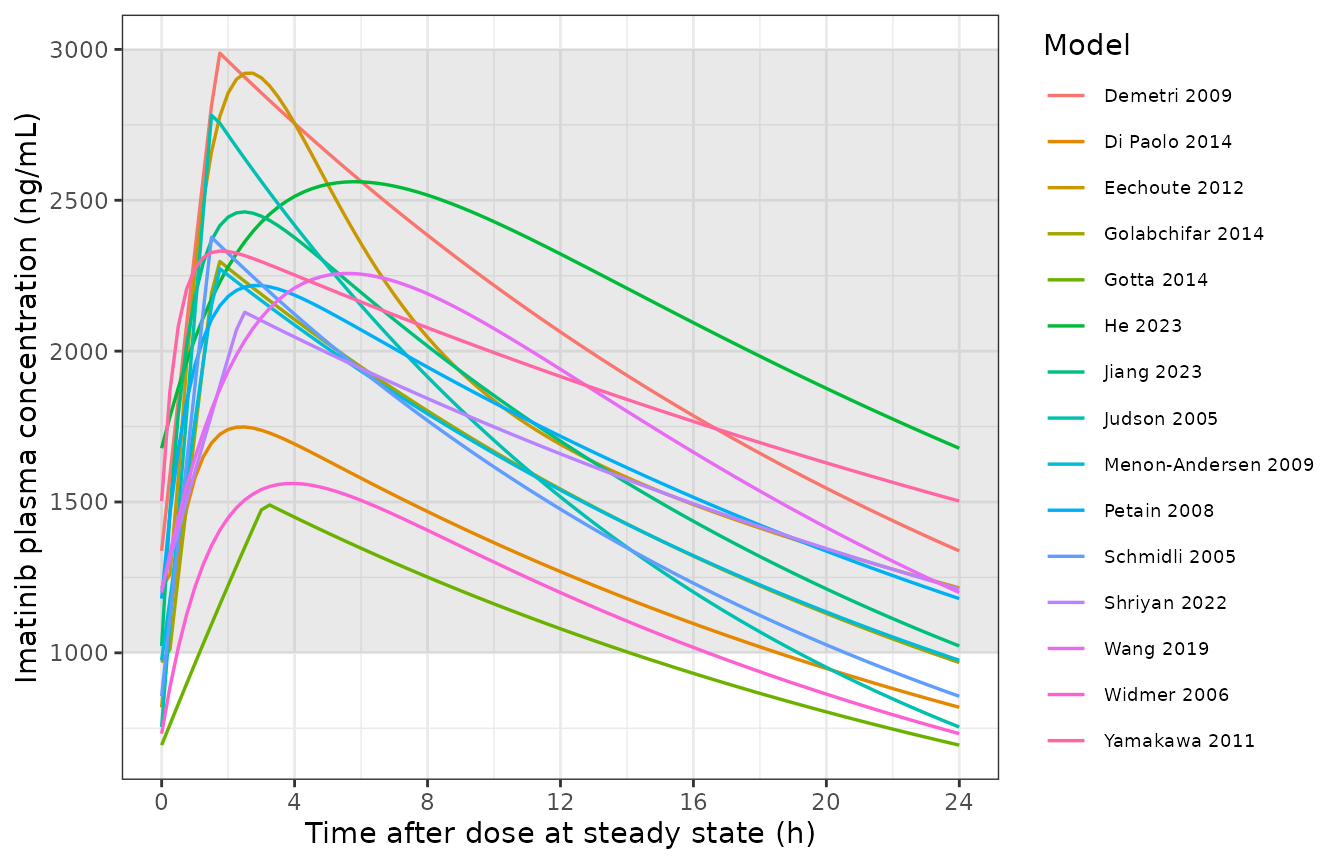

Steady-state imatinib concentration-time profiles over one 24 h dosing interval for the same reference subject on 400 mg once daily, predicted by each of the fifteen published models transcribed from Yang 2025 Table 1. The shaded band is the 1000-3000 ng/mL trough range recommended in the therapeutic-drug-monitoring literature that Yang 2025 cites.

trough_tbl <-
  sim_typ |>
  dplyr::filter(abs(time_rel - tau) < 1e-8) |>
  dplyr::transmute(label, cl = round(cl, 3), ctrough = round(Cc, 1)) |>
  dplyr::arrange(ctrough)

trough_tbl |>
  dplyr::rename(
    "Model" = label,
    "Clearance in the reference subject (L/h)" = cl,
    "Predicted steady-state trough (ng/mL)" = ctrough
  ) |>
  knitr::kable(caption = "Predicted 24 h steady-state trough concentration for one identical reference subject on imatinib 400 mg once daily, by model.")

Predicted 24 h steady-state trough concentration for one identical reference subject on imatinib 400 mg once daily, by model.

Model	Clearance in the reference subject (L/h)	Predicted steady-state trough (ng/mL)
Gotta 2014	15.831	694.1
Widmer 2006	14.300	732.1
Judson 2005	10.601	754.0
Di Paolo 2014	13.093	819.5
Schmidli 2005	11.127	856.1
Golabchifar 2014	10.800	967.8
Menon-Andersen 2009	10.800	975.3
Jiang 2023	9.720	1022.7
Petain 2008	9.774	1179.6
Wang 2019	9.250	1199.9
Shriyan 2022	10.200	1211.5
Eechoute 2012	9.120	1215.2
Demetri 2009	8.074	1337.7
Yamakawa 2011	8.700	1502.8
He 2023	7.600	1678.0

cat(sprintf(
  "Predicted trough spans %.0f to %.0f ng/mL, a %.1f-fold range across models.\n",
  min(trough_tbl$ctrough), max(trough_tbl$ctrough),
  max(trough_tbl$ctrough) / min(trough_tbl$ctrough)
))
#> Predicted trough spans 694 to 1678 ng/mL, a 2.4-fold range across models.

That fold-range is the quantitative form of Yang 2025’s conclusion. The fifteen models were fitted to different populations, different sampling designs and different assays, and they do not agree on the exposure that a single well-specified patient will achieve on the licensed dose. Yang 2025’s external evaluation found that none of them reached the pre-specified precision criterion (median absolute prediction error at or below 30%) on real TDM data, even after allometric scaling, and that the observations falling outside the 90% prediction interval were disproportionately from children.

Replicating the published typical-clearance range

Yang 2025 Results 3.1 states: “The typical apparent clearance was estimated to be 7.29-17.3 L/h.” That range is over the fifteen models’ typical values at their own reference covariate values, so it is an exact check on the transcribed lcl parameters, independent of everything else in the files.

typical_cl <- vapply(
  models,
  function(m) unname(exp(m$theta[["lcl"]])),
  numeric(1)
)

clearance_tbl <- tibble::tibble(
  label = model_specs$label,
  typical_cl = round(unname(typical_cl), 3)
) |>
  dplyr::arrange(typical_cl)

clearance_tbl |>
  dplyr::rename(
    "Model" = label,
    "Typical CL or CL/F at the model's own reference (L/h)" = typical_cl
  ) |>
  knitr::kable(caption = "Typical clearance parameter of each transcribed model. The minimum and maximum reproduce the 7.29-17.3 L/h range stated in Yang 2025 Results 3.1.")

Typical clearance parameter of each transcribed model. The minimum and maximum reproduce the 7.29-17.3 L/h range stated in Yang 2025 Results 3.1.

Model	Typical CL or CL/F at the model’s own reference (L/h)
Petain 2008	7.290
He 2023	7.600
Demetri 2009	8.180
Yamakawa 2011	8.700
Eechoute 2012	9.120
Wang 2019	9.250
Jiang 2023	9.720
Shriyan 2022	10.200
Judson 2005	10.600
Menon-Andersen 2009	10.800
Golabchifar 2014	10.800
Di Paolo 2014	13.093
Schmidli 2005	13.800
Widmer 2006	14.300
Gotta 2014	17.300

stopifnot(isTRUE(all.equal(min(typical_cl), 7.29, tolerance = 1e-6)))
stopifnot(isTRUE(all.equal(max(typical_cl), 17.3, tolerance = 1e-6)))
cat("Typical clearance range reproduces Yang 2025 Results 3.1 exactly: 7.29 to 17.3 L/h.\n")
#> Typical clearance range reproduces Yang 2025 Results 3.1 exactly: 7.29 to 17.3 L/h.

The minimum is Petain 2008 (the children-and-adults model) and the maximum is Gotta 2014 (the 2478-patient routine-care cohort). Note that Schmidli 2005’s lcl of 13.8 L/h is its day-1 value; on the day-29-or-later occasion used for TDM it falls to 10.62 L/h, which is why the trough table above and this table order the models differently.

PKNCA validation

Non-compartmental analysis is run on the simulated steady-state interval for every model. The structural identity available at steady state is exact and per-subject rather than a comparison of medians:

AUC(0-tau) x CL = F x Dose

Because the typical-value solve fixes every random effect, any departure from that identity is a coding error in the model file, in the dosing setup, or in the NCA window, not sampling noise. This is a much stronger test than comparing a simulated Cmax against a published one, and it is the only NCA check the source paper’s contents can support: Yang 2025 reports prediction-error metrics against its own undistributed dataset, not NCA parameters.

conc_data <-
  sim_typ |>
  dplyr::filter(!is.na(Cc)) |>
  dplyr::transmute(id, label, time = time_rel, Cc)

dose_data <-
  model_specs |>
  dplyr::transmute(id = 1L, label, time = 0, dose_amount = dose_mg)

# The model label is the treatment-like grouping variable and is listed before
# `id`; PKNCAdose() rejects a nested (slash) grouping formula, so both objects
# use the additive form.
o_conc <- PKNCA::PKNCAconc(conc_data, Cc ~ time | label + id,
                           concu = "ng/mL", timeu = "h")
o_dose <- PKNCA::PKNCAdose(dose_data, dose_amount ~ time | label + id,
                           doseu = "mg")

nca_intervals <- data.frame(
  start = 0, end = tau,
  auclast = TRUE, cmax = TRUE, tmax = TRUE, cmin = TRUE
)

o_data <- PKNCA::PKNCAdata(o_conc, o_dose, intervals = nca_intervals)
nca_res <- PKNCA::pk.nca(o_data)

nca_wide <-
  as.data.frame(nca_res) |>
  dplyr::select(label, PPTESTCD, PPORRES) |>
  tidyr::pivot_wider(names_from = PPTESTCD, values_from = PPORRES)

# Model-specific bioavailability. Only Eechoute 2012 carries an explicit F term
# (its `fdepot` variable); for every other model F is folded into the apparent
# CL/F and Vc/F, so F = 1 and bind_rows has left the column NA.
if (!("fdepot" %in% names(sim_typ))) sim_typ$fdepot <- NA_real_

f_by_model <-
  sim_typ |>
  dplyr::group_by(label) |>
  dplyr::summarise(
    cl = unique(round(cl, 8)),
    fdepot = if (all(is.na(fdepot))) 1 else unique(round(fdepot, 8)),
    .groups = "drop"
  )

identity_tbl <-
  nca_wide |>
  dplyr::left_join(f_by_model, by = "label") |>
  dplyr::mutate(
    # auclast is in ng/mL * h and cl in L/h, so their product is in ug;
    # divide by 1000 to reach the mg in which the dose is expressed.
    amount_recovered_mg = auclast * cl / 1000,
    expected_mg = fdepot * dose_mg,
    pct_error = 100 * (amount_recovered_mg - expected_mg) / expected_mg
  )

identity_tbl |>
  dplyr::transmute(
    label,
    auclast = round(auclast, 0),
    cmax = round(cmax, 0),
    tmax = round(tmax, 2),
    cmin = round(cmin, 0),
    pct_error = round(pct_error, 3)
  ) |>
  dplyr::arrange(label) |>
  dplyr::rename(
    "Model" = label,
    "AUC0-tau (ng*h/mL)" = auclast,
    "Cmax (ng/mL)" = cmax,
    "Tmax (h)" = tmax,
    "Cmin (ng/mL)" = cmin,
    "AUC x CL vs F x Dose, % error" = pct_error
  ) |>
  knitr::kable(caption = "Steady-state non-compartmental analysis of the reference subject on 400 mg once daily, with the mass-balance identity AUC0-tau x CL = F x Dose checked per model.")

Steady-state non-compartmental analysis of the reference subject on 400 mg once daily, with the mass-balance identity AUC0-tau x CL = F x Dose checked per model.

Model	AUC0-tau (ng*h/mL)	Cmax (ng/mL)	Tmax (h)	Cmin (ng/mL)	AUC x CL vs F x Dose, % error
Demetri 2009	49536	2988	1.75	1338	-0.013
Di Paolo 2014	30543	1749	2.50	820	-0.025
Eechoute 2012	43985	2921	2.75	1215	-0.001
Golabchifar 2014	37034	2297	1.75	968	-0.008
Gotta 2014	25264	1490	3.25	694	-0.009
He 2023	52629	2561	5.75	1678	-0.005
Jiang 2023	41141	2461	2.50	1023	-0.028
Judson 2005	37731	2782	1.50	754	-0.006
Menon-Andersen 2009	37031	2273	1.75	975	-0.016
Petain 2008	40917	2217	2.75	1180	-0.017
Schmidli 2005	35949	2377	1.50	856	-0.001
Shriyan 2022	39213	2129	2.50	1211	-0.007
Wang 2019	43240	2257	5.50	1200	-0.008
Widmer 2006	27968	1561	4.00	732	-0.014
Yamakawa 2011	45967	2332	1.75	1503	-0.022

# The identity is exact up to ODE solver tolerance and the trapezoidal
# approximation of AUC on a 0.25 h grid.
stopifnot(max(abs(identity_tbl$pct_error)) < 1)
cat(sprintf(
  "AUC(0-tau) x CL reproduces F x Dose for all %d models; worst absolute error %.3f%%.\n",
  nrow(identity_tbl), max(abs(identity_tbl$pct_error))
))
#> AUC(0-tau) x CL reproduces F x Dose for all 15 models; worst absolute error 0.028%.

The metabolite sub-models

Two of the fifteen models carry N-desmethyl imatinib (CGP74588) alongside the parent. Both parameterise the metabolite as apparent with respect to the fraction of imatinib metabolized to it (CLm/fm, V1m/fm, and for Menon-Andersen also Qm/fm and V2m/fm), because fm is not identifiable from plasma data alone. The central_ndmima state therefore holds an fm-scaled amount; the predicted metabolite concentration is nonetheless the true one, because the same fm divides both the clearance and the volume and cancels in their ratio.

met_stems <- structure_tbl$label[structure_tbl$metabolite]

sim_typ |>
  dplyr::filter(label %in% met_stems) |>
  dplyr::select(label, time_rel, Imatinib = Cc, `N-desmethyl imatinib` = Cc_ndmima) |>
  tidyr::pivot_longer(c(Imatinib, `N-desmethyl imatinib`),
                      names_to = "Analyte", values_to = "conc") |>
  ggplot(aes(x = time_rel, y = conc, colour = Analyte)) +
  geom_line(linewidth = 0.7) +
  facet_wrap(~label) +
  scale_x_continuous(breaks = seq(0, 24, by = 6)) +
  labs(x = "Time after dose at steady state (h)",
       y = "Plasma concentration (ng/mL)") +
  theme_bw()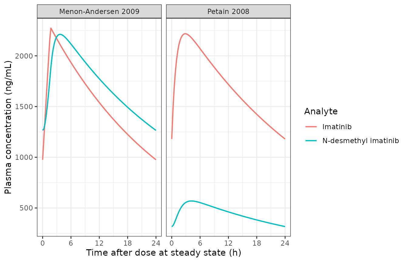

Parent imatinib and N-desmethyl imatinib steady-state profiles for the reference subject on 400 mg once daily, from the two models that carry the metabolite. Both were developed on cohorts that included children.

sim_typ |>
  dplyr::filter(label %in% met_stems, abs(time_rel - tau) < 1e-8) |>
  dplyr::transmute(
    label,
    parent = round(Cc, 1),
    metabolite = round(Cc_ndmima, 1),
    ratio_pct = round(100 * Cc_ndmima / Cc, 1)
  ) |>
  dplyr::rename(
    "Model" = label,
    "Imatinib trough (ng/mL)" = parent,
    "N-desmethyl imatinib trough (ng/mL)" = metabolite,
    "Metabolite-to-parent ratio (%)" = ratio_pct
  ) |>
  knitr::kable(caption = "Steady-state trough metabolite-to-parent ratio predicted by the two parent-metabolite models.")

Steady-state trough metabolite-to-parent ratio predicted by the two parent-metabolite models.

Model	Imatinib trough (ng/mL)	N-desmethyl imatinib trough (ng/mL)	Metabolite-to-parent ratio (%)
Petain 2008	1179.6	316.8	26.9
Menon-Andersen 2009	975.3	1264.9	129.7

Between-subject variability: a stochastic cohort

The typical-value work above deliberately holds every random effect at zero. The between-subject variability the models carry is large and differs markedly between them, which is the other half of why they disagree. A 200-subject cohort is simulated for three contrasting models: the smallest reported IIV on clearance (Jiang 2023, 13.9%), the largest single-parameter IIV among the one-compartment models (Golabchifar 2014, whose lag time carries 68.3%), and the 2478-patient routine-care model (Gotta 2014).

n_sub <- 200
vpc_stems <- c("Jiang_2023_imatinib", "Gotta_2014_imatinib", "Golabchifar_2014_imatinib")

solve_cohort <- function(stem) {
  mod <- models[[stem]]
  ev <- build_events(mod, obs_by = 0.5)
  params <- ref_covs[names(ref_covs) %in% mod$allCovs]

  set.seed(20250908)
  out <- rxode2::rxSolve(mod, ev, params = params, nSub = n_sub,
                         returnType = "data.frame")
  # With covariates supplied as a plain named vector and subjects generated by
  # nSub, rxSolve names the subject column `sim.id` rather than `id`. Normalise
  # it so the assertion below actually measures the simulated cohort size
  # instead of silently reading a missing column.
  out$id <- out$sim.id
  out$stem <- stem
  out$time_rel <- out$time - tau * (n_days - 1)
  out[out$time_rel >= 0, , drop = FALSE]
}

sim_vpc <-
  dplyr::bind_rows(lapply(vpc_stems, solve_cohort)) |>
  dplyr::left_join(model_specs[, c("stem", "label")], by = "stem")

stopifnot(dplyr::n_distinct(sim_vpc$id) == n_sub)

sim_vpc |>
  dplyr::group_by(label, time_rel) |>
  dplyr::summarise(
    p05 = quantile(Cc, 0.05),
    p50 = median(Cc),
    p95 = quantile(Cc, 0.95),
    .groups = "drop"
  ) |>
  ggplot(aes(x = time_rel)) +
  annotate("rect", xmin = -Inf, xmax = Inf, ymin = 1000, ymax = 3000,
           alpha = 0.12, fill = "grey30") +
  geom_ribbon(aes(ymin = p05, ymax = p95, fill = label), alpha = 0.25) +
  geom_line(aes(y = p50, colour = label), linewidth = 0.7) +
  facet_wrap(~label) +
  scale_x_continuous(breaks = seq(0, 24, by = 6)) +
  labs(x = "Time after dose at steady state (h)",
       y = "Imatinib plasma concentration (ng/mL)") +
  theme_bw() +
  theme(legend.position = "none")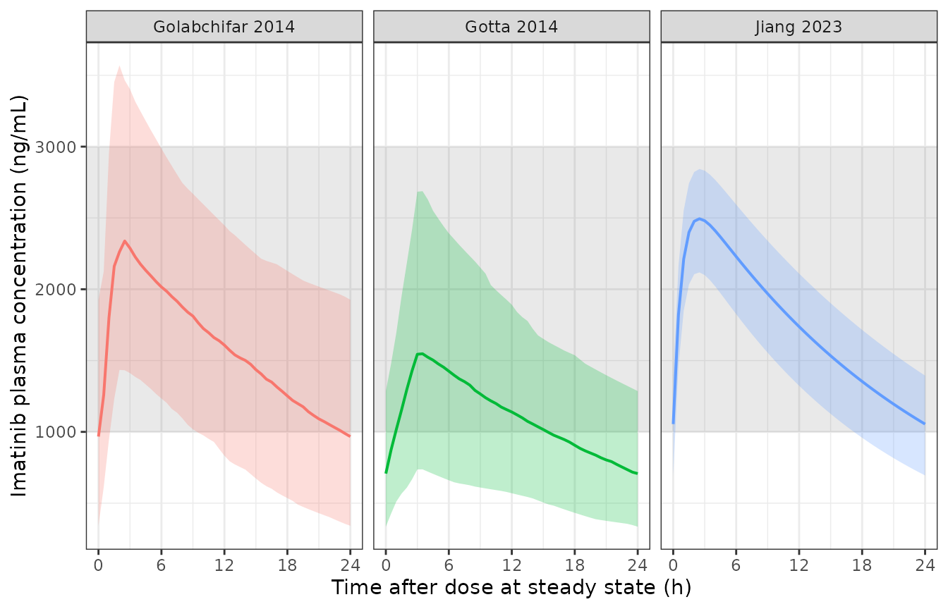

Simulated between-subject spread in steady-state imatinib concentrations for three contrasting models, 200 virtual subjects each sharing the reference subject’s covariates. Solid line is the median, ribbon spans the 5th to 95th percentiles. Only the random effects differ between subjects.

sim_vpc |>
  dplyr::filter(abs(time_rel - tau) < 1e-8) |>
  dplyr::group_by(label) |>
  dplyr::summarise(
    p05 = round(quantile(Cc, 0.05), 0),
    p50 = round(median(Cc), 0),
    p95 = round(quantile(Cc, 0.95), 0),
    in_window_pct = round(100 * mean(Cc >= 1000 & Cc <= 3000), 1),
    .groups = "drop"
  ) |>
  dplyr::rename(
    "Model" = label,
    "5th percentile trough (ng/mL)" = p05,
    "Median trough (ng/mL)" = p50,
    "95th percentile trough (ng/mL)" = p95,
    "Within the 1000-3000 ng/mL window (%)" = in_window_pct
  ) |>
  knitr::kable(caption = "Simulated steady-state trough distribution on 400 mg once daily for three models, 200 virtual subjects each. The final column is the fraction of subjects whose predicted trough falls inside the therapeutic-drug-monitoring window Yang 2025 cites.")

Simulated steady-state trough distribution on 400 mg once daily for three models, 200 virtual subjects each. The final column is the fraction of subjects whose predicted trough falls inside the therapeutic-drug-monitoring window Yang 2025 cites.

Model	5th percentile trough (ng/mL)	Median trough (ng/mL)	95th percentile trough (ng/mL)	Within the 1000-3000 ng/mL window (%)
Golabchifar 2014	342	967	1926	48.0
Gotta 2014	335	708	1286	16.5
Jiang 2023	695	1055	1394	57.0

The three models disagree not only on the typical trough but on how many patients a fixed 400 mg dose would place inside the target window. That is the practical case for TDM which Yang 2025 makes, and simultaneously the reason they conclude that model-based dose individualisation for imatinib is not yet reliable, particularly in children, for whom none of these cohorts provides real support.

Assumptions and deviations

Recorded here because the source is a secondary one, so the gaps are systematic rather than incidental.

1. Every parameter comes from Yang 2025 Table 1, not the primary. See the provenance section above. All fourteen new files should be re-extracted when their primaries are obtained.

2. CV% is converted as omega = CV/100. Settled mechanically by the Demetri 2009 covariance, which is inadmissible under the exact log-normal conversion. Judson 2005’s Var(...) entries are used as variances directly, settled by the same argument on its own covariance; Yamakawa 2011’s omega entries are squared.

3. Widmer 2006 carries no covariate. Yang 2025 Table 1 footnote c records that the evaluation used “the demographic base model”, so the alpha-1 acid glycoprotein relationship after which the primary is titled is not available from the secondary source. This is the largest single known gap between the transcription and its primary; it is documented in that file’s covariatesDataExcluded.

4. Demetri 2009 repeats its CL/F covariate exponents on Vc/F. Yang 2025 Table 1 prints (ALB/38.3)^1.66 x (WBC/7)^-0.418 on both parameters. This was checked against the original PDF with pdftotext -layout rather than the trimmed markdown, so it is genuinely what the secondary source prints and not a table-flattening artifact. It remains unusual and is the highest-priority item to confirm against the primary.

5. Eechoute 2012’s transit-chain topology is an inference. Table 1 gives the absorption model only as “T5” with rate constants Ktr and Ka and does not print the chain layout. A dosing depot followed by five transit compartments, with the final step into central at ka, is used. The alternative reading (dosing directly into transit1, with no separate depot) shortens the mean absorption time by one 1/ktr step, about 4% of the total, so the choice is numerically near-immaterial.

6. Eechoute 2012’s shared Vc-Ka random effect. Table 1 prints a single omega under the hyphenated label CV%(Vc-Ka), in contrast to the separate per-parameter entries on the same row. It is implemented as one eta multiplying both vc and ka. If the primary instead reports two separate omegas of equal magnitude, the correction is confined to that one term.

7. Gotta 2014’s variability on the residual-error magnitude is omitted. Table 1 reports CV%(sigma_Prop) = 36.2%, an inter-individual random effect on the size of the proportional residual error itself. nlmixr2’s error-model syntax provides no supported way to attach an eta to a residual SD, so this component is not encoded. Typical-value predictions, the covariate model and the CL/V random effects are unaffected; only the simulated between-subject spread in residual scatter is narrower than the published model implies.

8. He 2023’s renal covariate has an inferred upper branch. Table 1 footnote h is truncated: it gives theta_eGFR = (eGFR/85)^0.25 when eGFR is below 85 but prints no “else” clause. The value above the hinge is taken to be 1, the only reading that keeps the function continuous at the hinge and the standard form for a renal-impairment-only covariate.

9. Unit conversions applied at the call site. Schmidli 2005 and He 2023 use hemoglobin in g/dL (the canonical HGB column permits either unit and each file declares which it uses). Di Paolo 2014’s alpha-1 acid glycoprotein threshold is printed as 94 mg/dL and is tested as 0.94 g/L against the canonical AAG column. Eechoute 2012’s liver-metastasis coefficient is per cm^3 and is divided by 1000 against the canonical TUM_VOL column, which is carried in mm^3. Additive residual errors printed in mg/L (Schmidli 249 ng/mL, Demetri 4 ng/mL, Yamakawa 400 ng/mL) are converted to the ng/mL in which Cc is reported.

10. The occasion column is re-based. Yang 2025 Table 1 footnote b codes the source occasion as 0 (day 1) and 1 (day 29 or later). The canonical OCC column is 1-based, so the three affected models (Schmidli 2005, Petain 2008, Demetri 2009) map those to OCC = 1 and OCC = 2 respectively and decompose to a binary indicator inside model(). The occasion drives a typical-value shift, not inter-occasion random variability; no eta is attached to it.

11. The allometrically scaled variants are not encoded. Yang 2025 evaluated each adult-only model twice, once as published and once with standard allometric scaling substituted for the published weight terms. Only the as-published form is in this package, because the scaled variant is the reviewers’ modification rather than a published model.

12. The reference subject is a construction of this vignette. No single covariate vector is common to all fifteen cohorts, so the values in ref_covs were chosen to sit near the middle of the reported ranges and, where a model uses a threshold, on the reference side of it (AAG below Di Paolo’s 0.94 g/L cut point, CRCL above He’s 85 hinge, no liver metastases). A different reference subject would change the absolute troughs but not the finding of wide between-model dispersion.

13. Yang 2025 Table 3 is not reproduced. The prediction-error metrics (MDPE, MDAPE, F20, F30, RMSE) are computed against the authors’ own 39-patient TDM dataset, which is available only “from the corresponding author upon reasonable request” and is not distributed with the article.

Registry additions made alongside this extraction

• inst/references/compartment-names.md: the metabolite suffix ndmima (N-desmethyl imatinib, CGP74588), following the ndm<drug> contraction established by ndmsel.
• inst/references/covariate-columns.md: T_FIRSTDOSE (time elapsed since the first dose of a treatment course, hours) and SNP_SLC22A1_RS683369 (SLC22A1 / OCT1 c.480C>G L160F variant carrier indicator), both well-formed members of existing auto-approved canonical families.

Session information

sessionInfo()
#> R version 4.6.1 (2026-06-24)
#> Platform: x86_64-pc-linux-gnu
#> Running under: Ubuntu 24.04.4 LTS
#> 
#> Matrix products: default
#> BLAS:   /usr/lib/x86_64-linux-gnu/openblas-pthread/libblas.so.3 
#> LAPACK: /usr/lib/x86_64-linux-gnu/openblas-pthread/libopenblasp-r0.3.26.so;  LAPACK version 3.12.0
#> 
#> locale:
#>  [1] LC_CTYPE=C.UTF-8       LC_NUMERIC=C           LC_TIME=C.UTF-8       
#>  [4] LC_COLLATE=C.UTF-8     LC_MONETARY=C.UTF-8    LC_MESSAGES=C.UTF-8   
#>  [7] LC_PAPER=C.UTF-8       LC_NAME=C              LC_ADDRESS=C          
#> [10] LC_TELEPHONE=C         LC_MEASUREMENT=C.UTF-8 LC_IDENTIFICATION=C   
#> 
#> time zone: UTC
#> tzcode source: system (glibc)
#> 
#> attached base packages:
#> [1] stats     graphics  grDevices utils     datasets  methods   base     
#> 
#> other attached packages:
#> [1] ggplot2_4.0.3         dplyr_1.2.1           PKNCA_0.12.1         
#> [4] rxode2_5.1.6          nlmixr2lib_0.3.2.9000
#> 
#> loaded via a namespace (and not attached):
#>  [1] gtable_0.3.6        xfun_0.60           bslib_0.12.0       
#>  [4] lattice_0.22-9      vctrs_0.7.3         tools_4.6.1        
#>  [7] generics_0.1.4      parallel_4.6.1      tibble_3.3.1       
#> [10] symengine_0.2.13    pkgconfig_2.0.3     data.table_1.18.6.1
#> [13] checkmate_2.3.4     RColorBrewer_1.1-3  S7_0.2.2           
#> [16] desc_1.4.3          RcppParallel_6.2.1  lifecycle_1.0.5    
#> [19] compiler_4.6.1      farver_2.1.2        textshaping_1.0.5  
#> [22] fontawesome_0.5.3   htmltools_0.5.9     sys_3.4.3          
#> [25] sass_0.4.10         yaml_2.3.12         tidyr_1.3.2        
#> [28] pillar_1.11.1       pkgdown_2.2.1       crayon_1.5.3       
#> [31] jquerylib_0.1.4     whisker_0.4.1       openssl_2.4.2      
#> [34] cachem_1.1.0        nlme_3.1-169        tidyselect_1.2.1   
#> [37] digest_0.6.39       lotri_1.0.4         purrr_1.2.2        
#> [40] labeling_0.4.3      rxode2ll_2.0.16     fastmap_1.2.0      
#> [43] grid_4.6.1          cli_3.6.6           dparser_1.3.1-13   
#> [46] magrittr_2.0.5      withr_3.0.3         scales_1.4.0       
#> [49] backports_1.5.1     rmarkdown_2.31      otel_0.2.0         
#> [52] askpass_1.2.1       ragg_1.5.2          memoise_2.0.1      
#> [55] evaluate_1.0.5      knitr_1.51          rex_1.2.2          
#> [58] PreciseSums_0.7     rlang_1.3.0         downlit_0.4.5      
#> [61] Rcpp_1.1.2          glue_1.8.1          xml2_1.6.0         
#> [64] jsonlite_2.0.0      R6_2.6.1            systemfonts_1.3.2  
#> [67] fs_2.1.0