Ad26.COV2.S COVID-19 vaccine homologous booster antibody persistence (Dari 2023b)
Source:vignettes/articles/Dari_2023b_ad26cov2s.Rmd
Dari_2023b_ad26cov2s.RmdModel and source
- Citation: Dari A, Boulton M, Neyens M, Le Gars M, Valenzuela B, Shukarev G, Cardenas V, Ruiz-Guinazu J, Sadoff J, Hoetelmans RMW, Perez Ruixo JJ. Mechanistic modeling projections of antibody persistence after homologous booster regimens of COVID-19 vaccine Ad26.COV2.S in humans. CPT Pharmacometrics Syst Pharmacol. 2023;12(10):1485-1498. doi:10.1002/psp4.13025.
- Article: https://doi.org/10.1002/psp4.13025 (open access, PMC10583247)
Dari et al. pooled five Ad26.COV2.S trials (COV1001, COV1002, COV2001, COV3001, COV3009) in SARS-CoV-2-seronegative adults who received 5 x 10^10 viral particles (vp) either once or as a prime plus a homologous booster 2, 3 or 6 months later. They fit one mechanistic model of the humoral immune response jointly to the spike-binding antibody (S-ELISA, EU/mL) and the wild-type-virus neutralizing antibody (wtVNA, IC50 titer), and projected antibody persistence to 24 months.
The model extends the single-dose model of the same group
(Dari_2023_ad26cov2s_selisa, Clin Pharmacol Ther 2023) by
splitting the B-cell response into two pathways (Eq. 1-7, Figure 1):
- a K-PD virtual antigen compartment (
antigen), decaying atk_ag; - a memory-B-cell pathway (
bcell_memory, M1): antigen-driven and antigen-independent (kp_m) logistic growth ton_mem, differentiating into short-lived plasma cells (plasma_short) atkp_s * antigen; - a germinal-centre pathway (
germinal_center, M2): antigen-driven logistic growth ton_gc, differentiating into long-lived plasma cells (plasma_long) atkp_l * antigen; - antibody secretion (
kab_s,kab_l) into serum (antibody), distribution to a peripheral compartment (antibody_periph) and elimination (ke_ab).
The binding antibody is the output Cc. The neutralizing
titer wtvna is derived from it through a
neutralizing-to-binding ratio with a decaying IgM part (Eq. 8) and a
log10 slope (Eq. 9). Age lowers both antibody production rates and
female sex raises the long-lived-plasma-cell production rate.
mod <- readModelDb("Dari_2023b_ad26cov2s")
ui <- rxode2::rxode2(mod)
#> ℹ parameter labels from comments will be replaced by 'label()'
lloq <- c(selisa = 50.3, wtvna = 58) # Methods, 'Immunogenicity assays'
sd_s <- ui$theta[["expSd"]] # natural-log residual SD, S-ELISA
sd_v <- ui$theta[["expSd_wtvna"]] # natural-log residual SD, wtVNA
regimens <- c(
  "Single dose" = NA,
  "Booster (D1, D57)" = 56,
  "Booster (D1, D85)" = 84,
  "Booster (D1, D183)" = 182
)
Population
The analysis pooled 5,608 S-ELISA samples from 978 participants and
1,882 wtVNA samples from a subset of 375 participants, with data up to
15 months after the prime. From Table S1: the S-ELISA set had a median
age of 55 years (range 18-84; mean 52.2, SD 17.0), 48.6% women, 44.7%
aged >= 60 years, median weight 73.8 kg, and was 72.8% White
non-Hispanic, 12.3% Asian and 14.9% other race. The wtVNA subset had a
median age of 47 years (range 18-80), 45.9% women and 27.7% Asian
participants. Boosters were given on days 25-70 (2 months), 70-130 (3
months) or after day 130 (6 months). Participants who became infected
with SARS-CoV-2 were withdrawn from that point. The same information is
in the model’s population metadata.
Source trace
Every value is a Table 1 entry of Dari 2023b unless stated otherwise;
the in-file comments in
inst/modeldb/specificDrugs/Dari_2023b_ad26cov2s.R carry the
same trace.
| Parameter | Value | Source |
|---|---|---|
k_ag (1/day) |
0.065 (fixed) | Table 1 ‘kAg’ |
kp_ag (cells/antigen unit/day) |
1 (fixed) | Table 1 ‘kpAg’ |
kp_m (1/day) |
0.0167 | Table 1 ‘kpM’ |
ke_m, ke_gc (1/day) |
0 (fixed) | Table 1 ‘keM1 and keM2’ |
n_mem (cells) |
10.7 x 10^4 (fixed) | Table 1 ‘N1’ |
n_gc (cells) |
0.129 x 10^4 | Table 1 ‘N2’ |
kp_s, kp_l (1/day/antigen unit) |
0.5 x 10^-5 each (fixed) | Table 1 ‘kpS’, ‘kpL’ |
ke_s (1/day) |
0.578 (fixed) | Table 1 ‘keS’ |
ke_l (1/day) |
19.1 x 10^-4 | Table 1 ‘keL’; unit printed /year, see below |
kab_s, age 55 ((EU/mL)/cell/day) |
3.01 | Table 1 ‘kAbS’ |
kab_l, male aged 55 ((EU/mL)/cell/day) |
0.394 | Table 1 ‘kAbL’ |
kab_p, kp_ab, ke_ab
(1/day) |
0.2075, 0.2716, 0.0556 (fixed) | Table 1 |
alpha_wtvna |
0.732 | Table 1 ‘alpha’; Results ‘Correlation between S-ELISA and wtVNA’ |
beta_wtvna (IC50 per EU/mL) |
3.85 | Table 1 ‘beta’ |
igm_wtvna (IC50 per EU/mL) |
6.10 | Table 1 ‘IgM’ |
kigm (1/day) |
0.0368 | Table 1 ‘kIgM’ |
e_age_kab_s, e_age_kab_l
|
-0.221, -0.867 | Table 1; power model (AGE/55)^e, Appendix S1 ‘Covariate
analysis’ |
e_sexf_kab_l |
0.816 | Table 1; form kAbL * (1 + e * SEXF), Appendix S1 |
IIV kab_s, kab_l (CV) |
127%, 126% | Table 1; omega^2 = log(1 + CV^2) (footnote a) |
| Residual SD (log10 scale) | 0.21 (S-ELISA), 0.238 (wtVNA) | Table 1 ‘Proportional error’ (footnote c); Appendix S1 ‘Additive error model’ |
Antigen dose (amt) |
500 (x 10^8 vp) per dose | Not stated; see ‘Antigen dose scale’ |
| ODEs | Eq. 1-7 | Methods, ‘Structural model’ |
| wtVNA link | Eq. 8-9 | Methods, ‘Structural model’; see ‘Neutralizing-antibody link’ |
Shared helpers
# One dosing record per vaccination plus observation records. The model has
# two endpoints and neither is an ODE state, so observation rows carry
# dvid = 1 and no compartment; rxSolve still returns both Cc and wtvna.
make_events <- function(AGE, SEXF, boost, obs_times, amt = 500) {
  n <- length(AGE)
  covs <- data.frame(id = seq_len(n), AGE = AGE, SEXF = SEXF)
  dose_times <- c(0, boost[!is.na(boost)])
  dose <- expand.grid(time = dose_times, id = seq_len(n))
  dose$evid <- 1L
  dose$amt <- amt
  dose$cmt <- "antigen"
  dose$dvid <- NA_integer_
  obs <- expand.grid(time = obs_times, id = seq_len(n))
  obs$evid <- 0L
  obs$amt <- 0
  obs$cmt <- NA_character_
  obs$dvid <- 1L
  dplyr::bind_rows(dose, obs) |>
    dplyr::left_join(covs, by = "id") |>
    dplyr::arrange(id, time, dplyr::desc(evid))
}

# Age drawn from the Table S1 S-ELISA distribution (mean 52.2, SD 17.0,
# truncated to the observed 18-84 years), as the paper sampled age from the
# analysis dataset.
sample_age <- function(n, lower = 18, upper = 84) {
  out <- numeric(0)
  while (length(out) < n) {
    a <- rnorm(2 * n, 52.2, 17.0)
    out <- c(out, a[a >= lower & a <= upper])
  }
  out[seq_len(n)]
}

typical <- function(m, boost, times, amt = 500) {
  ev <- make_events(AGE = 55, SEXF = 0.5, boost = boost, obs_times = times, amt = amt)
  rxode2::rxSolve(rxode2::zeroRe(m), ev, returnType = "data.frame")
}
Antigen dose scale
Table 1 gives kp_ag in cells/vp/day and
kp_s, kp_l in 1/day/vp, but the paper never
states the number entered as the antigen dose. The same gap exists in
the single-dose paper, where 10^8 vp was the only power-of-ten unit that
reproduced the data. The maintainers repeated that check here: the
typical-value model (age 55, sex weight 0.5) was solved for each
power-of-ten unit of the nominal dose and compared with the simulated
medians of the Figure 3 VPC (black lines, digitised to about +/- 0.1
log10). Panel (d) is left out: its 6-month booster arm has about 15
participants whose boosters fall anywhere after day 130, so its
pre-booster bin is not a single-dose curve.
fig3_median <- tibble::tribble(
  ~regimen,            ~time, ~fig3_log10,
  "Single dose",          14, 2.27,
  "Single dose",          28, 2.60,
  "Single dose",          56, 2.72,
  "Single dose",          91, 2.78,
  "Single dose",         175, 2.60,
  "Single dose",         259, 2.62,
  "Booster (D1, D57)",    14, 2.22,
  "Booster (D1, D57)",    28, 2.55,
  "Booster (D1, D57)",    91, 3.37,
  "Booster (D1, D57)",   175, 3.15,
  "Booster (D1, D57)",   259, 2.93,
  "Booster (D1, D85)",    14, 2.30,
  "Booster (D1, D85)",    28, 2.60,
  "Booster (D1, D85)",   112, 3.35,
  "Booster (D1, D85)",   175, 3.07,
  "Booster (D1, D85)",   259, 2.98
)

dose_units <- c(
  "1e9 vp (amt = 50)" = 50,
  "1e8 vp (amt = 500)" = 500,
  "1e7 vp (amt = 5000)" = 5000,
  "vp (amt = 5e10)" = 5e10
)
scale_check <- dplyr::bind_rows(lapply(names(dose_units), function(u) {
  dplyr::bind_rows(lapply(unique(fig3_median$regimen), function(r) {
    typical(mod, regimens[[r]], sort(unique(fig3_median$time)), amt = dose_units[[u]]) |>
      dplyr::select(time, Cc) |>
      dplyr::mutate(regimen = r)
  })) |>
    dplyr::mutate(dose_unit = u)
})) |>
  dplyr::inner_join(fig3_median, by = c("regimen", "time")) |>
  dplyr::mutate(diff = log10(Cc) - fig3_log10)
#> ℹ parameter labels from comments will be replaced by 'label()'
#> ℹ omega/sigma items treated as zero: 'etalkab_s', 'etalkab_l'
#> ℹ parameter labels from comments will be replaced by 'label()'
#> ℹ omega/sigma items treated as zero: 'etalkab_s', 'etalkab_l'
#> ℹ parameter labels from comments will be replaced by 'label()'
#> ℹ omega/sigma items treated as zero: 'etalkab_s', 'etalkab_l'
#> ℹ parameter labels from comments will be replaced by 'label()'
#> ℹ omega/sigma items treated as zero: 'etalkab_s', 'etalkab_l'
#> ℹ parameter labels from comments will be replaced by 'label()'
#> ℹ omega/sigma items treated as zero: 'etalkab_s', 'etalkab_l'
#> ℹ parameter labels from comments will be replaced by 'label()'
#> ℹ omega/sigma items treated as zero: 'etalkab_s', 'etalkab_l'
#> ℹ parameter labels from comments will be replaced by 'label()'
#> ℹ omega/sigma items treated as zero: 'etalkab_s', 'etalkab_l'
#> ℹ parameter labels from comments will be replaced by 'label()'
#> ℹ omega/sigma items treated as zero: 'etalkab_s', 'etalkab_l'
#> ℹ parameter labels from comments will be replaced by 'label()'
#> ℹ omega/sigma items treated as zero: 'etalkab_s', 'etalkab_l'
#> ℹ parameter labels from comments will be replaced by 'label()'
#> ℹ omega/sigma items treated as zero: 'etalkab_s', 'etalkab_l'
#> ℹ parameter labels from comments will be replaced by 'label()'
#> ℹ omega/sigma items treated as zero: 'etalkab_s', 'etalkab_l'
#> ℹ parameter labels from comments will be replaced by 'label()'
#> ℹ omega/sigma items treated as zero: 'etalkab_s', 'etalkab_l'

scale_fit <- scale_check |>
  dplyr::group_by(dose_unit) |>
  dplyr::summarise(mean_abs_log10_diff = mean(abs(diff)), .groups = "drop")
scale_fit |>
  dplyr::rename("Dose unit" = dose_unit, "Mean |difference| (log10)" = mean_abs_log10_diff) |>
knitr::kable(digits = 2, caption = "Typical-value S-ELISA vs the Figure 3 VPC median, by candidate dose unit.")| Dose unit | Mean |difference| (log10) |
|---|---|
| 1e7 vp (amt = 5000) | 1.35 |
| 1e8 vp (amt = 500) | 0.09 |
| 1e9 vp (amt = 50) | 1.73 |
| vp (amt = 5e10) | 8.53 |
# Deterministic typical-value solves. Only the 10^8-vp unit lands within a
# few tenths of a log10 of the Figure 3 median; its neighbours miss by more
# than one log10.
fit_of <- function(u) scale_fit$mean_abs_log10_diff[scale_fit$dose_unit == u]
stopifnot(
  fit_of("1e8 vp (amt = 500)") < 0.2,
  fit_of("1e9 vp (amt = 50)") > 1,
  fit_of("1e7 vp (amt = 5000)") > 1,
  fit_of("vp (amt = 5e10)") > 1
)
Each 5 x 10^10 vp dose is therefore entered as
amt = 500.
Virtual cohorts
The main cohort has 200 participants per regimen, with age drawn as
above and a 1:1 sex ratio (the paper’s simulation design). Observations
are weekly to day 728 (26 four-week months), so the same solve serves
the VPC, the exploratory geometric means and the persistence rule.
Residual error is added on the log scale with the model’s own residual
SDs, giving Cc_obs and wtvna_obs.
rxode2::rxSetSeed(2023)
set.seed(2023)
n_arm <- 200
obs_days <- seq(0, 728, by = 7)

sim_regimen <- function(m, boost, AGE, SEXF) {
  rxode2::rxSolve(m, make_events(AGE, SEXF, boost, obs_days), returnType = "data.frame")
}
sim_main <- dplyr::bind_rows(lapply(names(regimens), function(r) {
  sim_regimen(mod, regimens[[r]], sample_age(n_arm), rep(0:1, length.out = n_arm)) |>
    dplyr::mutate(regimen = r)
})) |>
  dplyr::mutate(
    Cc_obs = Cc * exp(rnorm(dplyr::n(), 0, sd_s)),
    wtvna_obs = wtvna * exp(rnorm(dplyr::n(), 0, sd_v))
  )
#> ℹ parameter labels from comments will be replaced by 'label()'
stopifnot(all(c("AGE", "SEXF") %in% names(sim_main)))
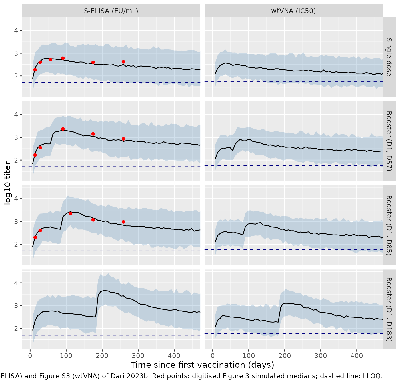
Figure 3 and Figure S3: visual predictive checks
vpc <- sim_main |>
  dplyr::filter(time > 0) |>
  tidyr::pivot_longer(c(Cc_obs, wtvna_obs), names_to = "assay", values_to = "value") |>
  dplyr::mutate(assay = ifelse(assay == "Cc_obs", "S-ELISA (EU/mL)", "wtVNA (IC50)")) |>
  dplyr::group_by(regimen, assay, time) |>
  dplyr::summarise(
    q05 = quantile(log10(value), 0.05),
    q50 = quantile(log10(value), 0.50),
    q95 = quantile(log10(value), 0.95),
    .groups = "drop"
  ) |>
  dplyr::mutate(regimen = factor(regimen, levels = names(regimens)))

ggplot(vpc, aes(time, q50)) +
  geom_ribbon(aes(ymin = q05, ymax = q95), fill = "steelblue", alpha = 0.25) +
  geom_line() +
  geom_point(
    data = fig3_median |> dplyr::mutate(assay = "S-ELISA (EU/mL)", regimen = factor(regimen, levels = names(regimens))),
    aes(time, fig3_log10), colour = "red"
  ) +
  geom_hline(
    data = data.frame(assay = c("S-ELISA (EU/mL)", "wtVNA (IC50)"), y = log10(lloq)),
    aes(yintercept = y), linetype = "dashed", colour = "navy"
  ) +
  facet_grid(regimen ~ assay) +
  coord_cartesian(xlim = c(0, 450)) +
  labs(
    x = "Time since first vaccination (days)", y = "log10 titer",
    caption = paste(
      "Replicates Figure 3 (S-ELISA) and Figure S3 (wtVNA) of Dari 2023b.",
      "Red points: digitised Figure 3 simulated medians; dashed line: LLOQ."
    )
  )
vpc_check <- vpc |>
  dplyr::filter(assay == "S-ELISA (EU/mL)") |>
  dplyr::mutate(regimen = as.character(regimen)) |>
  dplyr::inner_join(fig3_median, by = c("regimen", "time")) |>
  dplyr::mutate(diff = q50 - fig3_log10)
stopifnot(nrow(vpc_check) == nrow(fig3_median))
vpc_check |>
  dplyr::select(regimen, time, q50, fig3_log10, diff) |>
  dplyr::rename(
    "Regimen" = regimen, "Day" = time, "Simulated median" = q50,
    "Figure 3 median" = fig3_log10, "Difference" = diff
  ) |>
knitr::kable(digits = 2, caption = "Simulated vs digitised Figure 3 median (log10 EU/mL).")| Regimen | Day | Simulated median | Figure 3 median | Difference |
|---|---|---|---|---|
| Booster (D1, D57) | 14 | 2.30 | 2.22 | 0.08 |
| Booster (D1, D57) | 28 | 2.64 | 2.55 | 0.09 |
| Booster (D1, D57) | 91 | 3.30 | 3.37 | -0.07 |
| Booster (D1, D57) | 175 | 3.04 | 3.15 | -0.11 |
| Booster (D1, D57) | 259 | 2.82 | 2.93 | -0.11 |
| Booster (D1, D85) | 14 | 2.34 | 2.30 | 0.04 |
| Booster (D1, D85) | 28 | 2.66 | 2.60 | 0.06 |
| Booster (D1, D85) | 112 | 3.43 | 3.35 | 0.08 |
| Booster (D1, D85) | 175 | 3.14 | 3.07 | 0.07 |
| Booster (D1, D85) | 259 | 2.84 | 2.98 | -0.14 |
| Single dose | 14 | 2.36 | 2.27 | 0.09 |
| Single dose | 28 | 2.65 | 2.60 | 0.05 |
| Single dose | 56 | 2.75 | 2.72 | 0.03 |
| Single dose | 91 | 2.71 | 2.78 | -0.07 |
| Single dose | 175 | 2.54 | 2.60 | -0.06 |
| Single dose | 259 | 2.51 | 2.62 | -0.11 |
# The simulated median has a sampling SD of about 0.05 log10 at n = 200. A
# mis-transcribed production rate, dose or covariate shifts it by > 0.3.
stopifnot(
  abs(median(vpc_check$diff)) < 0.2,
  quantile(abs(vpc_check$diff), 0.9) < 0.3
)
The simulated medians run about 0.1 log10 below the Figure 3 medians after the peak. The paper’s VPC replays the observed design (actual booster days and the covariates of the participants sampled at each visit), which this simulation does not.
Neutralizing-antibody link (Eq. 8-9)
Eq. 8 defines the neutralizing-to-binding ratio
beta + IgM * exp(-kIgM * time) and Eq. 9 a log10 slope
alpha without intercept, but the paper does not write the
combined expression. Two compositions are possible:
- the slope applies to the ratio-adjusted level:
log10(wtVNA) = alpha * log10(ratio * Ab);
- the slope applies to the ratio-adjusted level:
- the ratio multiplies the slope-transformed level:
log10(wtVNA) = log10(ratio) + alpha * log10(Ab).
- the ratio multiplies the slope-transformed level:
The model uses (A). Figure 2b plots
log10(wtVNA / S-ELISA) over time since the first
vaccination, and the Supplementary Results give the observed wtVNA
geometric-mean peaks, so both readings can be checked against the paper
without fitting. Time in Eq. 8 is time since the first vaccination, as
in Figure 2b.
# Figure 2b medians (red solid line), digitised to about +/- 0.05.
fig2b <- tibble::tribble(
  ~time, ~fig2b_log_ratio,
  14, 0.00,
  28, -0.15,
  56, -0.28,
  91, -0.35,
  175, -0.35,
  259, -0.33,
  385, -0.30
)
alpha <- exp(ui$theta[["lalpha_wtvna"]])
beta <- exp(ui$theta[["lbeta_wtvna"]])
igm <- exp(ui$theta[["ligm_wtvna"]])
kigm <- exp(ui$theta[["lkigm"]])

link_cmp <- sim_main |>
  dplyr::filter(time %in% fig2b$time) |>
  dplyr::mutate(
    ratio = beta + igm * exp(-kigm * time),
    log_ratio_A = log10(wtvna) - log10(Cc),
    log_ratio_B = log10(ratio) + (alpha - 1) * log10(Cc)
  ) |>
  dplyr::group_by(time) |>
  dplyr::summarise(
    reading_A = median(log_ratio_A),
    reading_B = median(log_ratio_B),
    .groups = "drop"
  ) |>
  dplyr::inner_join(fig2b, by = "time")
knitr::kable(
  link_cmp |>
    dplyr::rename(
      "Day" = time, "(A) model" = reading_A, "(B) alternative" = reading_B,
      "Figure 2b" = fig2b_log_ratio
    ),
  digits = 2, caption = "Median log10(wtVNA / S-ELISA) by day since the first vaccination."
)| Day | (A) model | (B) alternative | Figure 2b |
|---|---|---|---|
| 14 | 0.01 | 0.24 | 0.00 |
| 28 | -0.14 | 0.07 | -0.15 |
| 56 | -0.25 | -0.07 | -0.28 |
| 91 | -0.35 | -0.19 | -0.35 |
| 175 | -0.33 | -0.18 | -0.35 |
| 259 | -0.34 | -0.19 | -0.33 |
| 385 | -0.28 | -0.13 | -0.30 |
# Reading (A) tracks Figure 2b to within a few hundredths of a log10;
# reading (B) sits 0.15-0.25 log10 too high at every visit. Both are medians
# of individual predictions over the same 800 participants, so the gap is
# stable across random draws.
stopifnot(
  mean(abs(link_cmp$reading_A - link_cmp$fig2b_log_ratio)) < 0.06,
  mean(abs(link_cmp$reading_B - link_cmp$fig2b_log_ratio)) > 0.12
)
Exploratory geometric means
The Results (‘S-ELISA and wtVNA geometric mean levels’) and the Supplementary Results report the observed geometric mean (GM) at the post-vaccination peak and 140-160 days after the second peak (days after the single peak for the single dose), with values below the LLOQ imputed to the LLOQ. The same summary is computed on the simulated observations.
gm_obs <- tibble::tribble(
  ~regimen,             ~assay,    ~paper_peak, ~paper_cth,
  "Single dose",        "S-ELISA",  543,  343,
  "Booster (D1, D57)",  "S-ELISA", 1760,  606,
  "Booster (D1, D85)",  "S-ELISA", 2056,  810,
  "Booster (D1, D183)", "S-ELISA", 2674, 1407,
  "Single dose",        "wtVNA",    271,  221,
  "Booster (D1, D57)",  "wtVNA",    584,  238,
  "Booster (D1, D85)",  "wtVNA",    854,  245,
  "Booster (D1, D183)", "wtVNA",    944,  582
)

gm_sim <- sim_main |>
  dplyr::filter(time > 0, time <= 450) |>
  tidyr::pivot_longer(c(Cc_obs, wtvna_obs), names_to = "assay", values_to = "value") |>
  dplyr::mutate(
    assay = ifelse(assay == "Cc_obs", "S-ELISA", "wtVNA"),
    value = pmax(value, ifelse(assay == "S-ELISA", lloq[["selisa"]], lloq[["wtvna"]]))
  ) |>
  dplyr::group_by(regimen, assay, time) |>
  dplyr::summarise(gm = exp(mean(log(value))), .groups = "drop") |>
  dplyr::left_join(
    data.frame(regimen = names(regimens), last_dose = ifelse(is.na(regimens), 0, regimens)),
    by = "regimen"
  ) |>
  dplyr::filter(time > last_dose) |>
  dplyr::group_by(regimen, assay) |>
  dplyr::summarise(
    sim_peak = max(gm),
    t_peak = time[which.max(gm)],
    sim_cth = gm[which.min(abs(time - (t_peak + 150)))],
    .groups = "drop"
  )

gm_cmp <- gm_obs |>
  dplyr::inner_join(gm_sim, by = c("regimen", "assay")) |>
  dplyr::mutate(
    peak_ratio = sim_peak / paper_peak,
    cth_ratio = sim_cth / paper_cth
  )
gm_cmp |>
  dplyr::select(regimen, assay, paper_peak, sim_peak, paper_cth, sim_cth) |>
  dplyr::rename(
    "Regimen" = regimen, "Assay" = assay, "Observed peak GM" = paper_peak,
    "Simulated peak GM" = sim_peak, "Observed GM 140-160 d after peak" = paper_cth,
    "Simulated GM 150 d after peak" = sim_cth
  ) |>
knitr::kable(digits = 0, caption = "Observed (Dari 2023b) vs simulated geometric means.")| Regimen | Assay | Observed peak GM | Simulated peak GM | Observed GM 140-160 d after peak | Simulated GM 150 d after peak |
|---|---|---|---|---|---|
| Single dose | S-ELISA | 543 | 603 | 343 | 345 |
| Booster (D1, D57) | S-ELISA | 1760 | 2113 | 606 | 783 |
| Booster (D1, D85) | S-ELISA | 2056 | 2597 | 810 | 703 |
| Booster (D1, D183) | S-ELISA | 2674 | 4957 | 1407 | 769 |
| Single dose | wtVNA | 271 | 379 | 221 | 206 |
| Booster (D1, D57) | wtVNA | 584 | 769 | 238 | 336 |
| Booster (D1, D85) | wtVNA | 854 | 845 | 245 | 304 |
| Booster (D1, D183) | wtVNA | 944 | 1286 | 582 | 361 |
# Observed GMs come from small, design-dependent subsets, so the check is on
# the centre of the ratios: a dose-scale or production-rate error moves every
# ratio by a factor of 3 or more. The 6-month booster arm (about 15
# participants from one study) is shown but not gated; see the text below.
gm_gate <- gm_cmp |> dplyr::filter(regimen != "Booster (D1, D183)")
log_ratios <- log10(c(gm_gate$peak_ratio, gm_gate$cth_ratio))
stopifnot(
  abs(median(log_ratios)) < 0.15,
  quantile(abs(log_ratios), 0.9) < 0.25
)
For the single dose and the 2- and 3-month boosters, the simulated geometric means agree with the observed ones to within about 40%. The 6-month booster arm does not: the simulated peak is about twice the observed one, and the level 150 days later is about half. That arm has about 15 participants (Results, ‘Projected persistence of humoral immune responses’). The paper’s own VPC (Figure 3d) replays those participants’ covariates, and its simulated median is about 3.0 log10 before the booster and 3.2 log10 at day 365, well above the typical curve of a 55-year-old. Covariates shift the post-booster curve by an amount of that order. The typical-value solve below shows this for a 30-year-old participant (sex weight 0.5), compared with the Figure 3d simulated median.
fig3d <- tibble::tribble(
  ~time, ~fig3d_log10,
  28, 2.72,
  175, 3.00,
  210, 3.52,
  365, 3.18
)
panel_d <- dplyr::bind_rows(
  typical(mod, 182, fig3d$time) |> dplyr::mutate(age = "55 years (reference)"),
  rxode2::rxSolve(
    rxode2::zeroRe(mod),
    make_events(AGE = 30, SEXF = 0.5, boost = 182, obs_times = fig3d$time),
    returnType = "data.frame"
  ) |> dplyr::mutate(age = "30 years")
) |>
  dplyr::select(age, time, Cc) |>
  dplyr::mutate(log10_Cc = log10(Cc)) |>
  dplyr::left_join(fig3d, by = "time")
#> ℹ parameter labels from comments will be replaced by 'label()'
#> ℹ omega/sigma items treated as zero: 'etalkab_s', 'etalkab_l'
#> ℹ parameter labels from comments will be replaced by 'label()'
#> ℹ omega/sigma items treated as zero: 'etalkab_s', 'etalkab_l'
panel_d |>
  dplyr::select(age, time, log10_Cc, fig3d_log10) |>
  dplyr::rename(
    "Age" = age, "Day" = time, "Typical log10 S-ELISA" = log10_Cc,
    "Figure 3d simulated median" = fig3d_log10
  ) |>
knitr::kable(digits = 2, caption = "6-month booster: typical-value S-ELISA by age vs Figure 3d.")| Age | Day | Typical log10 S-ELISA | Figure 3d simulated median |
|---|---|---|---|
| 55 years (reference) | 28 | 2.55 | 2.72 |
| 55 years (reference) | 175 | 2.52 | 3.00 |
| 55 years (reference) | 210 | 3.60 | 3.52 |
| 55 years (reference) | 365 | 2.82 | 3.18 |
| 30 years | 28 | 2.68 | 2.72 |
| 30 years | 175 | 2.74 | 3.00 |
| 30 years | 210 | 3.68 | 3.52 |
| 30 years | 365 | 3.04 | 3.18 |
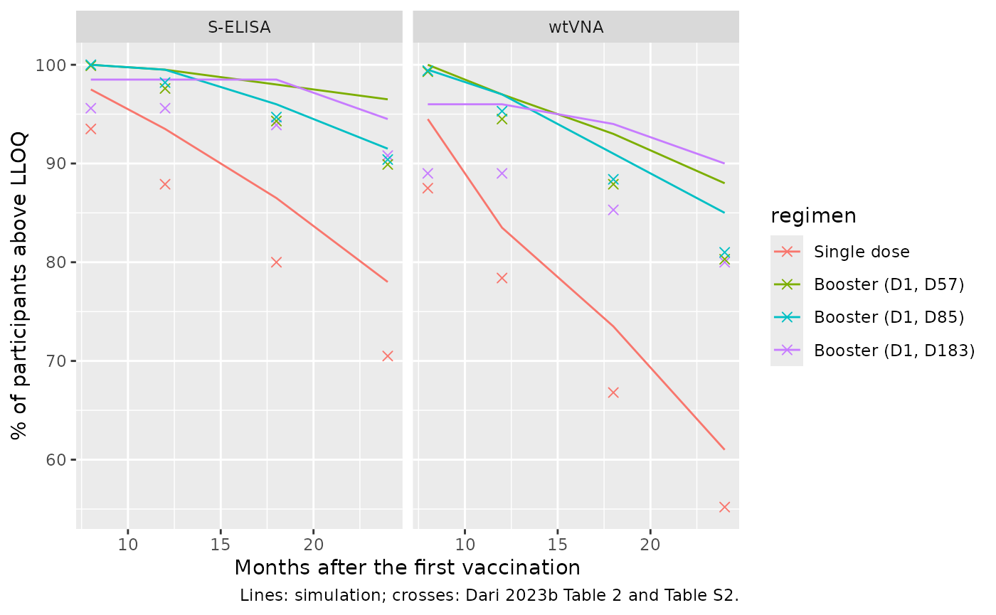
Table 2 and Table S2: persistence above the LLOQ
The paper defines individual persistence as the time from vaccination until the last titer above the LLOQ before two consecutive monthly titers below it, and reports the share of participants still persisting at 8, 12, 18 and 24 months. The simulation applies that rule to the four-weekly simulated observations (including residual error) of the main cohort.
month_days <- 28 * (1:26)
landmarks <- c(8, 12, 18, 24)

# Time of the first of two consecutive below-LLOQ titers; Inf if there is none.
first_below_pair <- function(time, below) {
  k <- which(below[-length(below)] & below[-1])
  if (length(k) == 0) Inf else time[k[1]]
}

persistence <- function(sim, ys, yv, by = "regimen") {
  sim |>
    dplyr::filter(time %in% month_days) |>
    dplyr::arrange(dplyr::across(dplyr::all_of(by)), id, time) |>
    dplyr::group_by(dplyr::across(dplyr::all_of(c(by, "id")))) |>
    dplyr::summarise(
      end_s = first_below_pair(time, .data[[ys]] < lloq[["selisa"]]),
      end_v = first_below_pair(time, .data[[yv]] < lloq[["wtvna"]]),
      .groups = "drop"
    ) |>
    tidyr::expand_grid(month = landmarks) |>
    dplyr::group_by(dplyr::across(dplyr::all_of(c(by, "month")))) |>
    dplyr::summarise(
      selisa = 100 * mean(end_s > month * 30.4375),
      wtvna = 100 * mean(end_v > month * 30.4375),
      .groups = "drop"
    )
}
# Predicted % above the LLOQ for the overall population, Dari 2023b Table 2
# (S-ELISA) and Table S2 (wtVNA). The 8-month row is day 239 in Table 2.
paper_pers <- tibble::tribble(
  ~regimen,             ~month, ~selisa, ~wtvna,
  "Single dose",             8,   93.5,   87.5,
  "Single dose",            12,   87.9,   78.4,
  "Single dose",            18,   80.0,   66.8,
  "Single dose",            24,   70.5,   55.2,
  "Booster (D1, D57)",       8,   99.9,   99.3,
  "Booster (D1, D57)",      12,   97.6,   94.5,
  "Booster (D1, D57)",      18,   94.3,   87.9,
  "Booster (D1, D57)",      24,   89.9,   80.3,
  "Booster (D1, D85)",       8,  100.0,   99.4,
  "Booster (D1, D85)",      12,   98.2,   95.3,
  "Booster (D1, D85)",      18,   94.7,   88.4,
  "Booster (D1, D85)",      24,   90.4,   81.0,
  "Booster (D1, D183)",      8,   95.6,   89.0,
  "Booster (D1, D183)",     12,   95.6,   89.0,
  "Booster (D1, D183)",     18,   93.9,   85.3,
  "Booster (D1, D183)",     24,   90.8,   80.0
) |>
  tidyr::pivot_longer(c(selisa, wtvna), names_to = "assay", values_to = "paper_pct")

pers_cmp <- persistence(sim_main, "Cc_obs", "wtvna_obs") |>
  tidyr::pivot_longer(c(selisa, wtvna), names_to = "assay", values_to = "sim_pct") |>
  dplyr::inner_join(paper_pers, by = c("regimen", "month", "assay")) |>
  dplyr::mutate(diff = sim_pct - paper_pct)
stopifnot(nrow(pers_cmp) == nrow(paper_pers))

pers_cmp |>
  dplyr::mutate(regimen = factor(regimen, levels = names(regimens))) |>
  dplyr::arrange(assay, regimen, month) |>
  dplyr::rename(
    "Assay" = assay, "Regimen" = regimen, "Month" = month,
    "Simulated %" = sim_pct, "Paper %" = paper_pct, "Difference" = diff
  ) |>
knitr::kable(digits = 1, caption = "Predicted percentage of participants with persisting titers above the LLOQ.")| Regimen | Month | Assay | Simulated % | Paper % | Difference |
|---|---|---|---|---|---|
| Single dose | 8 | selisa | 97.5 | 93.5 | 4.0 |
| Single dose | 12 | selisa | 93.5 | 87.9 | 5.6 |
| Single dose | 18 | selisa | 86.5 | 80.0 | 6.5 |
| Single dose | 24 | selisa | 78.0 | 70.5 | 7.5 |
| Booster (D1, D57) | 8 | selisa | 100.0 | 99.9 | 0.1 |
| Booster (D1, D57) | 12 | selisa | 99.5 | 97.6 | 1.9 |
| Booster (D1, D57) | 18 | selisa | 98.0 | 94.3 | 3.7 |
| Booster (D1, D57) | 24 | selisa | 96.5 | 89.9 | 6.6 |
| Booster (D1, D85) | 8 | selisa | 100.0 | 100.0 | 0.0 |
| Booster (D1, D85) | 12 | selisa | 99.5 | 98.2 | 1.3 |
| Booster (D1, D85) | 18 | selisa | 96.0 | 94.7 | 1.3 |
| Booster (D1, D85) | 24 | selisa | 91.5 | 90.4 | 1.1 |
| Booster (D1, D183) | 8 | selisa | 98.5 | 95.6 | 2.9 |
| Booster (D1, D183) | 12 | selisa | 98.5 | 95.6 | 2.9 |
| Booster (D1, D183) | 18 | selisa | 98.5 | 93.9 | 4.6 |
| Booster (D1, D183) | 24 | selisa | 94.5 | 90.8 | 3.7 |
| Single dose | 8 | wtvna | 94.5 | 87.5 | 7.0 |
| Single dose | 12 | wtvna | 83.5 | 78.4 | 5.1 |
| Single dose | 18 | wtvna | 73.5 | 66.8 | 6.7 |
| Single dose | 24 | wtvna | 61.0 | 55.2 | 5.8 |
| Booster (D1, D57) | 8 | wtvna | 100.0 | 99.3 | 0.7 |
| Booster (D1, D57) | 12 | wtvna | 97.0 | 94.5 | 2.5 |
| Booster (D1, D57) | 18 | wtvna | 93.0 | 87.9 | 5.1 |
| Booster (D1, D57) | 24 | wtvna | 88.0 | 80.3 | 7.7 |
| Booster (D1, D85) | 8 | wtvna | 99.5 | 99.4 | 0.1 |
| Booster (D1, D85) | 12 | wtvna | 97.0 | 95.3 | 1.7 |
| Booster (D1, D85) | 18 | wtvna | 91.0 | 88.4 | 2.6 |
| Booster (D1, D85) | 24 | wtvna | 85.0 | 81.0 | 4.0 |
| Booster (D1, D183) | 8 | wtvna | 96.0 | 89.0 | 7.0 |
| Booster (D1, D183) | 12 | wtvna | 96.0 | 89.0 | 7.0 |
| Booster (D1, D183) | 18 | wtvna | 94.0 | 85.3 | 8.7 |
| Booster (D1, D183) | 24 | wtvna | 90.0 | 80.0 | 10.0 |
ggplot(
  pers_cmp |> dplyr::mutate(regimen = factor(regimen, levels = names(regimens))),
  aes(month, sim_pct, colour = regimen)
) +
  geom_line() +
  geom_point(aes(y = paper_pct), shape = 4, size = 2) +
  facet_wrap(~assay, labeller = as_labeller(c(selisa = "S-ELISA", wtvna = "wtVNA"))) +
  labs(
    x = "Months after the first vaccination", y = "% of participants above LLOQ",
    caption = "Lines: simulation; crosses: Dari 2023b Table 2 and Table S2."
  )
# 200 participants per regimen give a sampling SD of 2-3 percentage points
# per cell, and the cells of one regimen move together because they share
# subjects. A 2,000-per-regimen run sits about 3 points above the paper (see
# the text below). A dose unit one power of ten off, or the alternative
# readings checked further down, move whole regimens by 10-25 points.
stopifnot(
  abs(median(pers_cmp$diff)) < 6,
  quantile(abs(pers_cmp$diff), 0.9) < 12
)
The simulated persistence follows Table 2 and Table S2 across regimens and reproduces the headline ordering: a steady decline after a single dose, and a 24-month persistence near 90% (S-ELISA) and 80-85% (wtVNA) after any booster. The simulation runs a few points high, by about 3 points in a 2,000-per-regimen run and most for the single dose and the 6-month booster arm. The paper also sampled parameter uncertainty, which widens the titer distribution and moves more participants below the LLOQ; this vignette simulates the point estimates only. The largest single gap is the 6-month booster at 8 months (paper 95.6% / 89.0%), which in the paper equals its 12-month value: those participants lost persistence before the booster, when only the prime had been given.
Figure 4: men aged 60 years and older
The paper’s most-quoted subgroup is men aged >= 60 years: 24-month persistence after a single dose of 50.7% (S-ELISA) and 34.3% (wtVNA), rising to at least 79.7% and 64.7% after any booster (Results, Figure 4).
rxode2::rxSetSeed(60)
set.seed(60)
sim_m60 <- dplyr::bind_rows(lapply(names(regimens), function(r) {
  sim_regimen(mod, regimens[[r]], sample_age(n_arm, lower = 60), rep(0, n_arm)) |>
    dplyr::mutate(regimen = r)
})) |>
  dplyr::mutate(
    eps_s = rnorm(dplyr::n()),
    eps_v = rnorm(dplyr::n()),
    Cc_obs = Cc * exp(sd_s * eps_s),
    wtvna_obs = wtvna * exp(sd_v * eps_v)
  )
m60 <- persistence(sim_m60, "Cc_obs", "wtvna_obs") |>
  dplyr::filter(month == 24)
m60 |>
  dplyr::mutate(regimen = factor(regimen, levels = names(regimens))) |>
  dplyr::arrange(regimen) |>
  dplyr::rename("Regimen" = regimen, "Month" = month, "S-ELISA %" = selisa, "wtVNA %" = wtvna) |>
knitr::kable(digits = 1, caption = "Simulated 24-month persistence, men aged >= 60 years.")| Regimen | Month | S-ELISA % | wtVNA % |
|---|---|---|---|
| Single dose | 24 | 54.5 | 40.0 |
| Booster (D1, D57) | 24 | 86.0 | 74.0 |
| Booster (D1, D85) | 24 | 87.5 | 70.5 |
| Booster (D1, D183) | 24 | 87.0 | 75.0 |
single60 <- m60[m60$regimen == "Single dose", ]
boost60 <- m60[m60$regimen != "Single dose", ]
# Across random draws each cell varies with an SD of about 5 points at
# n = 200, and the point-estimate simulation runs about 5 points above the
# paper here (see the persistence section). The check is on the mean of the
# four differences; the per-cell bound only catches a gross error. The
# alternative readings below move the single-dose cells by 10-35 points.
m60_diff <- c(
  single60$selisa - 50.7,
  single60$wtvna - 34.3,
  min(boost60$selisa) - 79.7,
  min(boost60$wtvna) - 64.7
)
stopifnot(
  abs(mean(m60_diff)) < 12,
  max(abs(m60_diff)) < 25
)
Readings not printed in the paper
Two Table 1 entries need a reading the paper does not spell out. Both were settled by the paper’s own persistence projections, which depend on them strongly; no value was fitted.
Long-lived plasma-cell elimination
ke_l. Table 1 prints 19.1 x 10^-4 with the unit
“year^-1”, the unit of the row above it. The single-dose paper estimated
16.8 x 10^-4 day^-1 for the same parameter. Read per year, the
long-lived plasma cells barely decline over 24 months (half-life 363
years), titers plateau and the single-dose persistence cannot fall from
93.5% to 70.5% as Table 2 reports.
Residual error scale. Appendix S1 states an additive error on log10 titers, while Table 1 labels the values “Proportional error” 21 (S-ELISA) and 23.8 (wtVNA) in a CV% column (footnote c: “refers to original values, i.e. additive error on log-transformed values”). The model reads them as log10-scale SDs x 100 (0.21 and 0.238), the reading that also fit the single-dose paper. Read as CVs on the original scale (natural-log SD 0.207 and 0.235) the residual noise around the LLOQ shrinks, and the persistence of men aged >= 60 years no longer falls as far as Figure 4 shows.
rxode2::rxSetSeed(7)
set.seed(7)
mod_kel_year <- mod |> rxode2::ini(lke_l = log(19.1e-4 / 365.25))
#> ℹ parameter labels from comments will be replaced by 'label()'
#> ℹ change initial estimate of `lke_l` to `-12.1612340875544`
sim_year <- sim_regimen(mod_kel_year, NA, sample_age(n_arm), rep(0:1, length.out = n_arm)) |>
  dplyr::mutate(
    regimen = "Single dose",
    Cc_obs = Cc * exp(rnorm(dplyr::n(), 0, sd_s)),
    wtvna_obs = wtvna * exp(rnorm(dplyr::n(), 0, sd_v))
  )
pers_year <- persistence(sim_year, "Cc_obs", "wtvna_obs")

# CV reading of the residual: same individual predictions and the same
# standard-normal draws as the men >= 60 cohort, smaller SDs.
sd_s_cv <- sqrt(log(1 + 0.21^2))
sd_v_cv <- sqrt(log(1 + 0.238^2))
m60_cv <- sim_m60 |>
  dplyr::mutate(
    Cc_cv = Cc * exp(sd_s_cv * eps_s),
    wtvna_cv = wtvna * exp(sd_v_cv * eps_v)
  ) |>
  persistence("Cc_cv", "wtvna_cv") |>
  dplyr::filter(month == 24, regimen == "Single dose")

readings <- tibble::tribble(
  ~check, ~assay, ~paper,
  "Single dose, 24 months, all", "S-ELISA", 70.5,
  "Single dose, 24 months, all", "wtVNA", 55.2,
  "Single dose, 24 months, men >= 60", "S-ELISA", 50.7,
  "Single dose, 24 months, men >= 60", "wtVNA", 34.3
) |>
  dplyr::mutate(
    model = c(
      pers_cmp$sim_pct[pers_cmp$regimen == "Single dose" & pers_cmp$month == 24 & pers_cmp$assay == "selisa"],
      pers_cmp$sim_pct[pers_cmp$regimen == "Single dose" & pers_cmp$month == 24 & pers_cmp$assay == "wtvna"],
      single60$selisa, single60$wtvna
    ),
    kel_per_year = c(
      pers_year$selisa[pers_year$month == 24], pers_year$wtvna[pers_year$month == 24],
      NA, NA
    ),
    residual_cv = c(NA, NA, m60_cv$selisa, m60_cv$wtvna)
  )
readings |>
  dplyr::rename(
    "Check" = check, "Assay" = assay, "Paper %" = paper, "Model %" = model,
    "keL read per year %" = kel_per_year, "Residual read as CV %" = residual_cv
  ) |>
knitr::kable(digits = 1, caption = "Persistence under the model's readings and the alternatives.")| Check | Assay | Paper % | Model % | keL read per year % | Residual read as CV % |
|---|---|---|---|---|---|
| Single dose, 24 months, all | S-ELISA | 70.5 | 78.0 | 92.5 | NA |
| Single dose, 24 months, all | wtVNA | 55.2 | 61.0 | 85.0 | NA |
| Single dose, 24 months, men >= 60 | S-ELISA | 50.7 | 54.5 | NA | 62 |
| Single dose, 24 months, men >= 60 | wtVNA | 34.3 | 40.0 | NA | 50 |
# keL per year leaves 24-month single-dose persistence above 90%, against
# 70.5% / 55.2% in the paper; the model sits within a few points. The CV
# reading overshoots the men >= 60 subgroup by about 8-12 points more than
# the log10 reading (same individuals, same draws).
stopifnot(
  readings$kel_per_year[1] - readings$paper[1] > 15,
  readings$kel_per_year[2] - readings$paper[2] > 15,
  mean(readings$residual_cv[3:4] - readings$model[3:4]) > 3
)
PKNCA: peak antibody response
The paper reports no non-compartmental analysis. This block computes the individual peak S-ELISA concentration after the last vaccination from the simulated individual predictions (no residual error) and compares its median with the observed geometric-mean peak of each regimen.
last_dose <- ifelse(is.na(regimens), 0, regimens)
nca_conc <- sim_main |>
  dplyr::filter(!is.na(Cc)) |>
  dplyr::mutate(id = paste(regimen, id)) |>
  dplyr::select(id, time, Cc, regimen)
stopifnot(all(nca_conc$time[!duplicated(nca_conc$id)] == 0))

nca_dose <- nca_conc |>
  dplyr::distinct(id, regimen) |>
  dplyr::left_join(data.frame(regimen = names(regimens), boost = regimens), by = "regimen") |>
  tidyr::expand_grid(dose_no = 1:2) |>
  dplyr::mutate(time = ifelse(dose_no == 1, 0, boost), amt = 500) |>
  dplyr::filter(!is.na(time)) |>
  dplyr::select(id, regimen, time, amt)

nca_int <- data.frame(
  regimen = names(regimens),
  start = unname(last_dose),
  end = unname(last_dose) + 150,
  cmax = TRUE,
  tmax = TRUE
)

nca_res <- PKNCA::pk.nca(PKNCA::PKNCAdata(
  PKNCA::PKNCAconc(nca_conc, Cc ~ time | regimen + id),
  PKNCA::PKNCAdose(nca_dose, amt ~ time | regimen + id),
  intervals = nca_int
))

nca_sim <- as.data.frame(nca_res) |>
  dplyr::filter(PPTESTCD %in% c("cmax", "tmax")) |>
  dplyr::select(regimen, PPTESTCD, PPORRES)
nca_ref <- data.frame(
  regimen = gm_obs$regimen[gm_obs$assay == "S-ELISA"],
  cmax = gm_obs$paper_peak[gm_obs$assay == "S-ELISA"]
)
nca_tbl <- nlmixr2lib::ncaComparisonTable(
  nca_sim |> dplyr::filter(PPTESTCD == "cmax"),
  nca_ref,
  by = "regimen",
  units = c(cmax = "EU/mL")
)
knitr::kable(nca_tbl, caption = "Median simulated S-ELISA Cmax after the last vaccination vs the observed geometric-mean peak.")| NCA parameter | regimen | Reference | Simulated | % diff |
|---|---|---|---|---|
| Cmax (EU/mL) | Single dose | 543 | 597 | +9.9% |
| Cmax (EU/mL) | Booster (D1, D57) | 1760 | 1980 | +12.7% |
| Cmax (EU/mL) | Booster (D1, D85) | 2060 | 2630 | +28.1%* |
| Cmax (EU/mL) | Booster (D1, D183) | 2670 | 4830 | +80.5%* |
nca_sim |>
  dplyr::group_by(regimen, PPTESTCD) |>
  dplyr::summarise(median = median(PPORRES), .groups = "drop") |>
  tidyr::pivot_wider(names_from = PPTESTCD, values_from = median) |>
  dplyr::mutate(regimen = factor(regimen, levels = names(regimens))) |>
  dplyr::arrange(regimen) |>
  dplyr::rename("Regimen" = regimen, "Median Cmax (EU/mL)" = cmax, "Median Tmax (day after last dose)" = tmax) |>
knitr::kable(digits = 0, caption = "Simulated peak S-ELISA response.")| Regimen | Median Cmax (EU/mL) | Median Tmax (day after last dose) |
|---|---|---|
| Single dose | 597 | 56 |
| Booster (D1, D57) | 1984 | 28 |
| Booster (D1, D85) | 2635 | 28 |
| Booster (D1, D183) | 4828 | 21 |
- differs from reference by more than ±20%.
The single-dose and 2-month booster peaks agree with the observed
geometric means to within about 15%, and the 3-month booster peak is
about 30% higher. The 6-month booster peak is well above the observed
2,674 EU/mL, for the reasons given under ‘Exploratory geometric means’:
in the model, memory B cells keep expanding between the prime and the
booster (kp_m, with no memory-B-cell loss), so a later
booster meets a larger memory pool. The paper reports a 4.92-fold rise
in peak S-ELISA concentration after a 6-month booster, but that observed
rise comes from a small arm with its own covariate mix.
Assumptions and deviations
-
Antigen dose scale (not stated in the paper). Each
vaccine dose enters the K-PD antigen compartment as
amt = 500, i.e. 5 x 10^10 vp in units of 10^8 vp. The paper giveskp_ag,kp_sandkp_lper vp but never the amount entered. The maintainers compared each power-of-ten unit of the nominal dose and kept the only one that reproduces Figure 3 (see above). No continuous fitting was done. -
ke_lunit. Table 1 prints the long-lived plasma-cell elimination rate 19.1 x 10^-4 with unit year^-1; the model reads it per day, as in the single-dose paper, because the per-year reading cannot produce the persistence decline of Table 2 and Table S2. -
Residual error scale. The Table 1 “Proportional
error” entries are read as log10-scale SDs x 100 and encoded as
lnorm()SDs on the natural-log scale (0.4835 and 0.5480), consistent with Appendix S1 and with the single-dose paper. -
wtVNA link. Eq. 8 and Eq. 9 are composed as
log10(wtVNA) = alpha * log10((beta + IgM * exp(-kIgM * t)) * Ab), the composition that reproduces Figure 2b. Time in the IgM term is time since the first vaccination, so a simulation must start at the prime. - Age effect. Appendix S1 gives the continuous covariate model as a power of the covariate over its median (55 years). The Results quote decreases of 23% (kAbS) and 64% (kAbL) between 23 and 84 years; the power model gives 25% and 68% over that range (the quoted figures match a lower percentile of about 26 years). The printed equation is kept.
- Persistence simulation. The paper simulated 250,000 participants with parameter uncertainty; this vignette uses 200 participants per regimen and the point estimates. Age is drawn from a normal distribution with the Table S1 mean and SD truncated to 18-84 years.
-
Observation names. The binding-antibody output is
named
Cc, as in the single-dose model and inDasti_2025_mrna1273_qsp, although it is an antibody response and not a concentration of the administered vaccine. The neutralizing titer iswtvna. -
Screened covariates. Body weight, race and country
were screened and not retained; body weight is listed in
covariatesDataExcluded. - No erratum or correction notice for Dari 2023b was found in Europe PMC as of 2026-10-27.