Empagliflozin exposure-response (Riggs 2014)
Source:vignettes/articles/Riggs_2014_empagliflozin.Rmd
Riggs_2014_empagliflozin.RmdModel and source
- Citation: Riggs MM, Seman LJ, Staab A, MacGregor TR, Gillespie W, Gastonguay MR, Woerle HJ, Macha S. Exposure-response modelling for empagliflozin, a sodium glucose cotransporter 2 (SGLT2) inhibitor, in patients with type 2 diabetes. Br J Clin Pharmacol. 2014;78(6):1407-1418. doi:10.1111/bcp.12453. The allometric exponents and the 70 kg reference weight of the PK layer are not printed in Riggs 2014 (which states only that ‘weight was included allometrically on each of these parameters’); they are taken from the companion population PK paper whose model Riggs 2014 uses: Riggs MM, Staab A, Seman L, MacGregor TR, Bergsma TT, Gastonguay MR, Macha S. Population pharmacokinetics of empagliflozin, a sodium glucose cotransporter 2 inhibitor, in patients with type 2 diabetes. J Clin Pharmacol. 2013;53(10):1028-1038. doi:10.1002/jcph.147 (Table 3: CL/F and Q/F scale as (WT/70)^0.75 FIXED; V2/F and V3/F as (WT/70)^1 FIXED).
- Description: Exposure-response (E-R) model for empagliflozin in patients with type 2 diabetes mellitus (T2DM), linking steady-state exposure to 24 h urinary glucose excretion (UGE), fasting plasma glucose (FPG) and HbA1c (Riggs 2014 Br J Clin Pharmacol). The PK layer is the two-compartment, lagged-first-order-absorption population PK model whose parameter values Riggs 2014 restates in Results, with an imposed allometric body-weight effect. The dosing-interval AUC (AUCss = DOSE_EMPA_MGD * 1e6 / MW / CL) drives a single stimulation function STIM that simultaneously lowers FPG and raises UGE. UGE is an algebraic sum of an exponential baseline in FPG and a saturable drug term (Umax, Ustim50); FPG is a turnover state whose removal is enhanced by STIM; FPG in turn drives first-order HbA1c production against a physiologic-limit boundary. Study-specific baselines and study-specific UGE / potency factors are carried for all five contributing studies (A-E). Data: 974 T2DM patients, 1-100 mg once daily, up to 12 weeks, from five randomised placebo-controlled trials.
- Article: https://doi.org/10.1111/bcp.12453
- Companion population PK paper (source of the allometric exponents and the 70 kg reference weight): https://doi.org/10.1002/jcph.147
Riggs 2014 links empagliflozin exposure to three glycaemic endpoints
through a single stimulation function STIM.
STIM rises hyperbolically with the dosing-interval AUC, is
amplified by the patient’s baseline fasting plasma glucose (FPG), and
simultaneously (a) enhances the removal of FPG and (b) drives a
saturable increase in 24 h urinary glucose excretion (UGE). FPG in turn
drives first-order HbA1c production against a physiologic-limit
boundary.
Population
The exposure-response analysis pooled 974 patients with type 2 diabetes from five randomised, placebo-controlled, once-daily trials (Riggs 2014 Table 1): two phase I studies in Germany (study A, n = 48, 8 days; study B, n = 78, 4 weeks), one phase II study in Japan enrolling only Japanese patients (study C, n = 100, 4 weeks), and two 12-week multinational phase IIb studies (study D, n = 324 analysed, empagliflozin monotherapy; study E, n = 424, on background metformin). Open-label metformin (study D) and open-label sitagliptin (study E) arms were excluded. Doses spanned 1 to 100 mg once daily.
Patients were 41 % female with a mean age of 57 to 58 years by study. Body weight differed markedly across studies: the Japanese cohort of study C averaged 67.9 kg against 81.4 to 94.6 kg elsewhere, which Riggs 2014 cites as a partial explanation for that study’s greater low-dose response. Baseline FPG study means were 8.3 to 9.7 mmol/L (overall range 2.8 to 21.0) and baseline HbA1c study means 7.1 to 8.1 % (range 5.6 to 10.4). Renal function was largely preserved: creatinine clearance study means were 94 to 117 mL/min and fewer than 1.5 % of patients had a value below 50 mL/min.
The same information is available programmatically via
readModelDb("Riggs_2014_empagliflozin")()$population.
Source trace
Every ini() entry carries an in-file comment naming its
origin; the table collects them for review. “Table 2” and “Results”
refer to Riggs 2014 unless noted.
| Equation / parameter | Value | Source location |
|---|---|---|
d/dt(depot), d/dt(central),
d/dt(peripheral1), alag(depot)
|
n/a | Results, “Empagliflozin exposures were estimated from a population PK model that included two compartmental disposition with lagged first order absorption and first order elimination (Figure 3)” |
lcl |
9.87 L/h | Results, PK paragraph |
lvc |
3.02 L | Results, PK paragraph |
lvp |
60.4 L | Results, PK paragraph |
lq |
5.16 L/h | Results, PK paragraph |
lka |
0.224 1/h | Results, PK paragraph |
lalag |
0.5 h, FIXED | Results, “Following a 0.5 h lag”; FIXED per Riggs 2013 Table 3 |
e_wt_cl, e_wt_q
|
0.75, FIXED |
Not in Riggs 2014 (which says only “weight was
included allometrically on each of these parameters”); Riggs 2013 Table
3 rows CL/F (WT/70)^theta_20 and
Q/F (WT/70)^theta_22, both FIXED |
e_wt_vc, e_wt_vp
|
1, FIXED |
Not in Riggs 2014; Riggs 2013 Table 3 rows
V2/F (WT/70)^theta_21 and
V3/F (WT/70)^theta_23, both FIXED |
etalcl, etalvp, etalka
|
CV 26.9 %, 30.8 %, 15.2 % | Results, PK paragraph; back-transformed as
omega^2 = log(1 + CV^2)
|
auc (exposure driver) |
n/a | Methods, “AUC_i,j (AUC of the dosing interval for each individual following each dose time in each study) was used for efficacy E-R evaluation”; MW 450.9 g/mol from Results |
uge (Equation 1) |
n/a | Equation 1, p. 1411 |
luge_base |
3.71 g/24 h | Table 2 theta_12 |
lf_uge_base_b, lf_uge_base_c
|
0.320, 0.632 | Table 2 theta_20, theta_16 |
lgamma_base, lf_gamma_base_c
|
5.31, 1.16 | Table 2 theta_13, theta_17 |
lumax, lf_umax_c
|
121 g/24 h, 1.11 | Table 2 theta_10, theta_14 |
lustim50, lf_ustim50_c
|
0.590, 1.58 | Table 2 theta_11, theta_15 |
etaluge_base |
CV 158.4 % | Results, “IIV for baseline UGE (CV%) was estimated to be 158.4%” |
stim (Equation 2) |
n/a | Equation 2, p. 1411 |
emax_trunc, beta_fpg,
gamma_fpg
|
0.0701, 0.795, 1.47 | Table 2 theta_6, theta_8, theta_9 |
lc50star |
498, FIXED | Table 2 theta_7 (RSE column reads FIXED) |
lf_c50star_c, lf_c50star_e
|
0.169, 1.93 | Table 2 theta_19, theta_21 |
d/dt(glucose) (Equation 3) |
n/a | Equation 3, p. 1412 – sign corrected, see Errata |
lkfpgout |
0.0407 1/h | Table 2 theta_5 |
fpg_base_a .. fpg_base_e
|
7.85, 8.50, 8.76, 9.30, 9.49 mmol/L | Table 2 theta_1, theta_2, theta_18, theta_3, theta_4 |
d/dt(hba1c) (Equation 4) |
n/a | Equation 4, p. 1412 |
lkhba1cout |
0.167 /week -> /168 | Table 2 theta_26 |
lkhba1cin |
0.078 %/week/mmol/L -> /168 | Table 2 theta_27 |
hba1c_limit |
3.34 % | Table 2 theta_22 |
eta_share |
2.7 | Table 2 theta_29
(eta_kHbA1c,out = theta_29 * eta_kHbA1c,in) |
lhba1c_base, lhba1c_base_c,
lhba1c_base_d, lhba1c_base_e
|
7.18, 7.85, 7.85, 7.89 % | Table 2 theta_23, theta_28, theta_24, theta_25 |
etalhba1c_base, etalkhba1cin,
covariance |
CV 9.53 %, CV 8.23 %, rho = -0.310 | Results, HbA1c paragraph |
expSd_uge, expSd_glucose,
expSd_hba1c
|
sqrt(0.380), sqrt(0.01461), sqrt(0.001287) | Table 2 “Residual variance” block |
WT allometric reference 70 kg |
70 kg | Riggs 2013 Table 3 and Figure 3 legend (“body weight of 70 kg”) |
ref_fpg = 8 mmol/L |
8 mmol/L | Equations 1 and 2; Results, “normalized to a FPG value of 8 mM (144 mg dl-1)” |
mw_empa = 450.9 g/mol |
450.9 | Results, “(molecular weight = 450.9 g mol-1)” |
Reparameterisation identities
Riggs 2014 estimated the FPG stimulation in an estimation-stable reparameterisation and reported the interpretable pair in the Table 2 “Calculated parameters” block. Both identities are reproduced exactly by the packaged model, which is the first check that the transcription is right.
mod  <- readModelDb("Riggs_2014_empagliflozin")
mod0 <- rxode2::zeroRe(mod)
#> ℹ parameter labels from comments will be replaced by 'label()'

# One typical subject, one study, one dose level, run to steady state.
solve_typical <- function(dose_mg, fpg_base, study = "A", wt = 70,
                          days = 220, obs_by = 24, extra = NULL) {
  ind <- c(A = 0, B = 0, C = 0, D = 0, E = 0)
  ind[study] <- 1
  ev <-
    rxode2::et(amt = dose_mg, ii = 24, until = days * 24, cmt = "depot") |>
    rxode2::et(seq(0, days * 24, by = obs_by), cmt = "glucose")
  ev <- as.data.frame(ev)
  ev$WT <- wt
  ev$DOSE_EMPA_MGD <- dose_mg
  ev$STUDY_EMPA_A <- ind[["A"]]
  ev$STUDY_EMPA_B <- ind[["B"]]
  ev$STUDY_EMPA_C <- ind[["C"]]
  ev$STUDY_EMPA_D <- ind[["D"]]
  ev$STUDY_EMPA_E <- ind[["E"]]
  # Riggs 2014 reports typical-subject predictions as a function of BASELINE
  # FPG, which in the model is a study-specific fixed effect. Overriding the
  # study A theta is the transparent way to evaluate the published model at an
  # arbitrary baseline; nothing else in the model changes.
  rxode2::rxSolve(
    mod0, ev,
    params = c(fpg_base_a = fpg_base, extra),
    returnType = "data.frame", omega = NA, sigma = NA
  )
}

ss <- function(...) {
  out <- solve_typical(...)
  out[nrow(out), ]
}

reparam <- tibble::tibble(
  Quantity = c("Emax (FPG maximal decrease, proportional)",
               "AUC50, studies A + B + D (nmol*h/L)",
               "AUC50, study C (nmol*h/L)",
               "AUC50, study E (nmol*h/L)",
               "HbA1c change per 1 mmol/L FPG at steady state (%)"),
  Model = c(ss(10, 7.85)$emax_fpg,
            ss(10, 7.85)$auc50,
            ss(10, 8.76, "C")$auc50,
            ss(10, 9.49, "E")$auc50,
            0.078 / 0.167),
  Published = c(0.158, 626, 106, 1210, 0.47),
  Source = c("Table 2, Calculated parameters", "Table 2, Calculated parameters",
             "Table 2, Calculated parameters", "Table 2, Calculated parameters",
             "Discussion, Samtani-style steady-state slope")
)

knitr::kable(reparam, digits = 4,
caption = "Reparameterisation identities reproduced from the packaged model.")| Quantity | Model | Published | Source |
|---|---|---|---|
| Emax (FPG maximal decrease, proportional) | 0.1583 | 0.158 | Table 2, Calculated parameters |
| AUC50, studies A + B + D (nmol*h/L) | 626.4151 | 626.000 | Table 2, Calculated parameters |
| AUC50, study C (nmol*h/L) | 105.8642 | 106.000 | Table 2, Calculated parameters |
| AUC50, study E (nmol*h/L) | 1208.9811 | 1210.000 | Table 2, Calculated parameters |
| HbA1c change per 1 mmol/L FPG at steady state (%) | 0.4671 | 0.470 | Discussion, Samtani-style steady-state slope |
# Deterministic typical-value identities: these must be tight.
stopifnot(
  abs(reparam$Model[1] - 0.158) < 5e-4,
  abs(reparam$Model[2] - 626) < 1,
  abs(reparam$Model[3] - 106) < 1,
  abs(reparam$Model[4] - 1210) < 2,
  abs(reparam$Model[5] - 0.47) < 5e-3
)
An independent structural check on the PK layer: the four disposition parameters imply a terminal half-life that the paper states only as “approximately 12 h” (Results, sourced to data on file).
Virtual cohort
The original patient-level data are not public. Two cohorts are used below.
The typical-subject cohort is a grid of doses,
studies and baseline FPG values solved with the random effects zeroed
(rxode2::zeroRe()); it is used to reproduce the exact
numbers Riggs 2014 prints for a typical patient.
The stochastic cohort below draws 100 subjects per treatment arm for the two 12-week studies (D and E), with body weight sampled to match the Table 1 means and standard deviations, and is used for the dose-response figures.
# set.seed() seeds R's RNG only. rxode2's simulation RNG is partitioned per
# solver thread, so the drawn cohort differs between a 2-core CI runner and a
# 16-thread workstation. Every assertion below is written on the centre or a
# robust quantile of the cohort, never on its extremes.
set.seed(20140626)

n_per_arm <- 100L

make_arm <- function(study, dose_mg, wt_mean, wt_sd, id_offset) {
  ind <- c(A = 0, B = 0, C = 0, D = 0, E = 0)
  ind[study] <- 1
  subj <- tibble::tibble(
    id = id_offset + seq_len(n_per_arm),
    WT = pmax(45, pmin(150, stats::rnorm(n_per_arm, wt_mean, wt_sd)))
  )
  # One compressed dose record per subject (ii = 24 h, 84 doses = 12 weeks)
  doses <- subj |>
    dplyr::mutate(time = 0, amt = dose_mg, evid = 1L, ii = 24, addl = 83L,
                  cmt = "depot")
  obs <- tidyr::expand_grid(
    subj,
    time = seq(0, 12 * 7 * 24, by = 7 * 24)   # weekly, 12 weeks
  ) |>
    dplyr::mutate(amt = 0, evid = 0L, ii = 0, addl = 0L, cmt = "glucose")
  dplyr::bind_rows(doses, obs) |>
    dplyr::mutate(
      study = study,
      arm = if (dose_mg == 0) "Placebo" else paste0(dose_mg, " mg"),
      DOSE_EMPA_MGD = dose_mg,
      STUDY_EMPA_A = ind[["A"]], STUDY_EMPA_B = ind[["B"]],
      STUDY_EMPA_C = ind[["C"]], STUDY_EMPA_D = ind[["D"]],
      STUDY_EMPA_E = ind[["E"]]
    ) |>
    dplyr::arrange(id, time, dplyr::desc(evid))
}

arms <- dplyr::bind_rows(
  # Study D: empagliflozin monotherapy, 5 / 10 / 25 mg or placebo (Methods)
  make_arm("D",  0, 81.4, 17, id_offset =    0L),
  make_arm("D",  5, 81.4, 17, id_offset =  100L),
  make_arm("D", 10, 81.4, 17, id_offset =  200L),
  make_arm("D", 25, 81.4, 17, id_offset =  300L),
  # Study E: on background metformin, 1 / 5 / 10 / 25 / 50 mg or placebo
  make_arm("E",  0, 89.2, 16, id_offset =  400L),
  make_arm("E",  1, 89.2, 16, id_offset =  500L),
  make_arm("E",  5, 89.2, 16, id_offset =  600L),
  make_arm("E", 10, 89.2, 16, id_offset =  700L),
  make_arm("E", 25, 89.2, 16, id_offset =  800L),
  make_arm("E", 50, 89.2, 16, id_offset =  900L)
)

stopifnot(
  !anyDuplicated(dplyr::distinct(arms[arms$evid == 0, c("id", "time")])),
  dplyr::n_distinct(arms$id) == 10L * n_per_arm
)Replicate published figures
Figure 1A - dose-response for urinary glucose excretion
Riggs 2014 Figure 1A shows observed 24 h UGE on study days 1 and 27
for the three studies that collected urine (A, B and C). The model
reproduction below is the typical-subject prediction at each study’s own
baseline FPG and its own UGE parameter set. Study C carries its own
value for all four UGE parameters and for C*50, which is
what makes its low-dose response so much steeper.
uge_grid <- tidyr::expand_grid(
  study = c("A", "B", "C"),
  dose = c(0, 1, 2.5, 5, 10, 25, 50, 100)
) |>
  dplyr::mutate(fpg_base = dplyr::recode(study, A = 7.85, B = 8.50, C = 8.76))
uge_grid$uge <- NA_real_
uge_grid$fpg_ss <- NA_real_
for (i in seq_len(nrow(uge_grid))) {
  r <- ss(uge_grid$dose[i], uge_grid$fpg_base[i], uge_grid$study[i])
  uge_grid$uge[i] <- r$uge
  uge_grid$fpg_ss[i] <- r$glucose
}
ggplot(uge_grid, aes(dose + 0.5, uge, colour = study)) +
  geom_line() +
  geom_point() +
  scale_x_log10(breaks = c(0.5, 1.5, 3, 5.5, 10.5, 25.5, 50.5, 100.5),
                labels = c("0", "1", "2.5", "5", "10", "25", "50", "100")) +
  labs(x = "Empagliflozin once-daily dose (mg)",
       y = "Predicted 24 h UGE (g)", colour = "Study",
       title = "Figure 1A - steady-state dose-response for urinary glucose excretion",
       caption = paste("Replicates the model prediction underlying Figure 1A of Riggs 2014.",
                       "The plateau between 10 and 25 mg is the paper's headline finding."))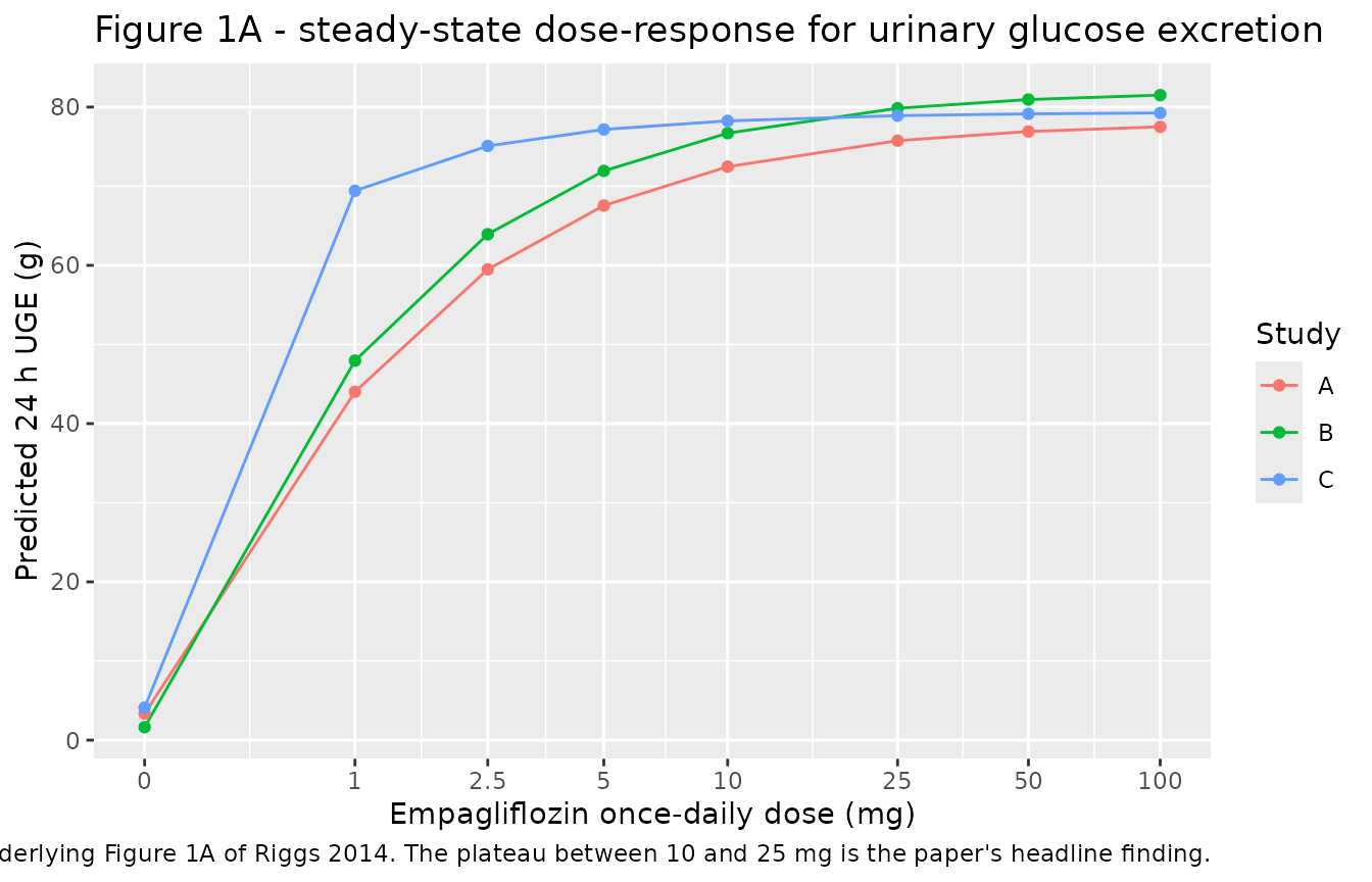
The paper reports the plateau in words: “An increase in UGE appeared to occur with the lowest dose of empagliflozin, with a dose-dependent increase in UGE thereafter, reaching a plateau at approximately 10 to 25 mg.”
plateau <- uge_grid |>
  dplyr::group_by(study) |>
  dplyr::summarise(
    monotone = all(diff(uge[order(dose)]) > 0),
    `10 mg as pct of 100 mg` = 100 * uge[dose == 10] / uge[dose == 100],
    `25 mg as pct of 100 mg` = 100 * uge[dose == 25] / uge[dose == 100],
    .groups = "drop"
  )
knitr::kable(plateau, digits = 1,
caption = "Approach to the UGE plateau by study.")| study | monotone | 10 mg as pct of 100 mg | 25 mg as pct of 100 mg |
|---|---|---|---|
| A | TRUE | 93.5 | 97.7 |
| B | TRUE | 94.1 | 98.0 |
| C | TRUE | 98.7 | 99.6 |
stopifnot(
  # UGE is monotone increasing in dose in every study.
  all(plateau$monotone),
  # "reaching a plateau at approximately 10 to 25 mg": 10 mg is already
  # within 10 pct of the 100 mg response and 25 mg within 5 pct.
  all(plateau$`10 mg as pct of 100 mg` > 90),
  all(plateau$`25 mg as pct of 100 mg` > 95)
)
Results-text predictions for UGE
Riggs 2014 quotes several typical-subject UGE increases.
Those are the drug-related term of Equation 1 alone, which the packaged
model exposes as uge_drug.
uge_pred <- tibble::tibble(
  Scenario = c("3 mg, baseline FPG 8 mmol/L",
               "10 mg, baseline FPG 8 mmol/L",
               "25 mg, baseline FPG 8 mmol/L",
               "3 mg, baseline FPG 10.5 mmol/L"),
  Model = c(ss(3, 8)$uge_drug, ss(10, 8)$uge_drug,
            ss(25, 8)$uge_drug, ss(3, 10.5)$uge_drug),
  Published = c(60, 72, 75, 80),
  Source = "Results, UGE paragraph"
)
knitr::kable(uge_pred, digits = 2,
caption = "Drug-related increase in 24 h UGE (g), typical subject, study A.")| Scenario | Model | Published | Source |
|---|---|---|---|
| 3 mg, baseline FPG 8 mmol/L | 61.13 | 60 | Results, UGE paragraph |
| 10 mg, baseline FPG 8 mmol/L | 72.02 | 72 | Results, UGE paragraph |
| 25 mg, baseline FPG 8 mmol/L | 75.44 | 75 | Results, UGE paragraph |
| 3 mg, baseline FPG 10.5 mmol/L | 79.44 | 80 | Results, UGE paragraph |
stopifnot(
  # The two two-significant-figure values are exact to the printed precision;
  # the "approximately 60" and "approximately 80" claims carry one.
  abs(uge_pred$Model[2] - 72) < 0.5,
  abs(uge_pred$Model[3] - 75) < 0.5,
  abs(uge_pred$Model[1] - 60) < 2,
  abs(uge_pred$Model[4] - 80) < 2,
  # Half of Umax (121 g/24 h) is reached at about the 3 mg exposure, which is
  # the paper's stated interpretation of the 626 nmol*h/L AUC50.
  abs(uge_pred$Model[1] / 121 - 0.5) < 0.06
)
The placebo baseline term is reported separately: UGE “was approximately doubled (e.g. from 2 to 4 to 8 to 16 g day-1) with baseline FPG increases from 8 mM to 9.1 mM, 10.4 mM and 11.8 mM”, and reaches “approximately 32 g day-1 for an FPG of 12 mM”.
base_fpg <- c(8, 9.1, 10.4, 11.8, 12)
base_uge <- vapply(base_fpg, function(b) ss(0, b)$uge, numeric(1))
baseline_tbl <- tibble::tibble(
  `Baseline FPG (mmol/L)` = base_fpg,
  `Predicted UGE (g/24 h)` = base_uge,
  `Fold vs 8 mmol/L` = base_uge / base_uge[1]
)
knitr::kable(baseline_tbl, digits = 2,
caption = "Placebo UGE baseline as a function of FPG, study A.")| Baseline FPG (mmol/L) | Predicted UGE (g/24 h) | Fold vs 8 mmol/L |
|---|---|---|
| 8.0 | 3.71 | 1.00 |
| 9.1 | 7.35 | 1.98 |
| 10.4 | 14.94 | 4.03 |
| 11.8 | 29.22 | 7.88 |
| 12.0 | 31.95 | 8.61 |
Figure 4 - relationship of UGE with FPG
Figure 4 plots 24 h UGE against FPG with one predicted line per treatment. The reproduction sweeps baseline FPG across the observed range and reads the steady-state FPG and UGE for each dose level.
fig4_grid <- tidyr::expand_grid(
  fpg_base = seq(5, 14, by = 0.5),
  dose = c(0, 1, 2.5, 5, 10, 25, 100)
)
fig4_grid$fpg <- NA_real_
fig4_grid$uge <- NA_real_
for (i in seq_len(nrow(fig4_grid))) {
  r <- ss(fig4_grid$dose[i], fig4_grid$fpg_base[i])
  fig4_grid$fpg[i] <- r$glucose
  fig4_grid$uge[i] <- r$uge
}
fig4_grid$treatment <- factor(
  ifelse(fig4_grid$dose == 0, "Placebo", paste0(fig4_grid$dose, " mg")),
  levels = c("Placebo", "1 mg", "2.5 mg", "5 mg", "10 mg", "25 mg", "100 mg")
)

ggplot(fig4_grid, aes(fpg, uge, colour = treatment)) +
  geom_line() +
  coord_cartesian(xlim = c(4, 14), ylim = c(0, 200)) +
  labs(x = "Fasting plasma glucose (mmol/L)", y = "24 h urinary glucose excretion (g)",
       colour = "Treatment",
       title = "Figure 4 - urinary glucose excretion vs fasting plasma glucose",
       caption = "Replicates the population-predicted lines of Figure 4 of Riggs 2014.")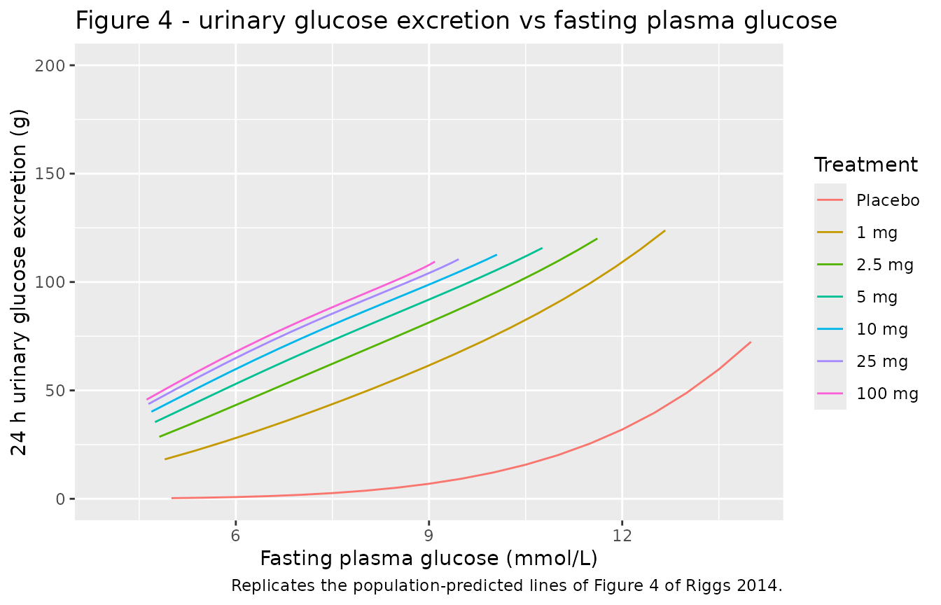
The paper’s reading of this figure is that “the relationship with FPG is retained with empagliflozin treatment, such that the magnitude of glucose removal (UGE) decreased as FPG decreased, thereby providing a degree of self-correction against hypoglycaemia”: every line rises with FPG, and the drug lines sit above placebo at every FPG.
by_trt <- split(fig4_grid, fig4_grid$treatment)
stopifnot(
  # Every treatment line is monotone increasing in FPG.
  all(vapply(by_trt, function(d) all(diff(d$uge[order(d$fpg)]) > 0), logical(1))),
  # Every drug line lies above placebo at matched baseline FPG.
  all(vapply(by_trt[-1], function(d) all(d$uge > by_trt[["Placebo"]]$uge), logical(1)))
)
Maximal steady-state FPG and HbA1c decreases
This is the paper’s most quantitative typical-subject claim and the
strongest transcription check available: four baseline FPG values, each
with a published maximal FPG decrease and a published maximal HbA1c
decrease (Results, FPG / HbA1c paragraph). A very large dose is used to
drive STIM to its asymptote.
maxdose <- 1e4  # far beyond the studied range; drives AUC >> AUC50
base_vals <- c(8, 7.4, 9.1, 10)
maxdec <- tibble::tibble(
  `Baseline FPG (mmol/L)` = base_vals,
  `FPG decrease, model (mmol/L)` =
    vapply(base_vals, function(b) ss(0, b)$glucose - ss(maxdose, b)$glucose, numeric(1)),
  `FPG decrease, published` = c(1.3, 1.0, 1.7, 2.2),
  `HbA1c decrease, model (pct pts)` =
    vapply(base_vals, function(b) ss(0, b)$hba1c - ss(maxdose, b)$hba1c, numeric(1)),
  `HbA1c decrease, published` = c(0.6, 0.5, 0.81, 1.0)
)
knitr::kable(maxdec, digits = 3,
caption = "Maximal steady-state decreases; published values from Riggs 2014 Results.")| Baseline FPG (mmol/L) | FPG decrease, model (mmol/L) | FPG decrease, published | HbA1c decrease, model (pct pts) | HbA1c decrease, published |
|---|---|---|---|---|
| 8.0 | 1.266 | 1.3 | 0.588 | 0.60 |
| 7.4 | 1.044 | 1.0 | 0.485 | 0.50 |
| 9.1 | 1.740 | 1.7 | 0.808 | 0.81 |
| 10.0 | 2.197 | 2.2 | 1.020 | 1.00 |
stopifnot(
  # Each model value rounds to the published value at the precision printed.
  all(abs(maxdec$`FPG decrease, model (mmol/L)` -
            maxdec$`FPG decrease, published`) < 0.05),
  all(abs(maxdec$`HbA1c decrease, model (pct pts)` -
            maxdec$`HbA1c decrease, published`) < 0.025),
  # 16 pct maximal proportional decrease at the 8 mmol/L reference.
  abs(maxdec$`FPG decrease, model (mmol/L)`[1] / 8 - 0.158) < 0.002
)
Figures 1B and 2 - dose-response for FPG and HbA1c
Figure 1B (FPG) and Figure 2 (HbA1c at weeks 4, 8 and 12) show the observed change from baseline by dose. The stochastic cohort reproduces the dose-response and the time course.
chg <- sim |>
  dplyr::filter(!is.na(glucose)) |>
  dplyr::group_by(id) |>
  dplyr::mutate(dfpg = glucose - dplyr::first(glucose),
                dhba1c = hba1c - dplyr::first(hba1c)) |>
  dplyr::ungroup() |>
  dplyr::mutate(week = time / (7 * 24),
                arm = factor(arm, levels = c("Placebo", "1 mg", "5 mg",
                                             "10 mg", "25 mg", "50 mg")))

chg |>
  dplyr::filter(week %in% c(4, 8, 12)) |>
  ggplot(aes(arm, dhba1c, fill = study)) +
  geom_boxplot(outlier.size = 0.5) +
  geom_hline(yintercept = 0, linetype = "dashed", colour = "grey50") +
  geom_hline(yintercept = -0.6, linetype = "dotted", colour = "darkgreen") +
  facet_wrap(~week, labeller = label_both) +
  labs(x = "Empagliflozin once-daily dose", y = "Change in HbA1c from baseline (pct pts)",
       fill = "Study",
       title = "Figure 2 - HbA1c dose-response at weeks 4, 8 and 12",
       caption = paste("Replicates Figure 2 of Riggs 2014;",
                       "reference lines at 0 and -0.6 percentage points."))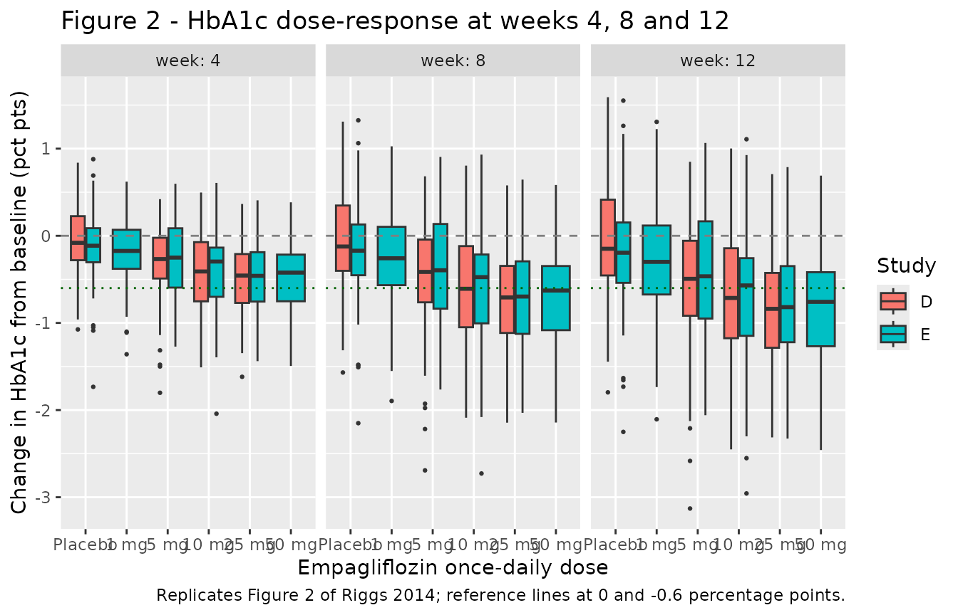
chg |>
  dplyr::filter(week == 12) |>
  ggplot(aes(arm, dfpg, fill = study)) +
  geom_boxplot(outlier.size = 0.5) +
  geom_hline(yintercept = c(2.5, 1.25, 0, -1.25, -2.5), colour = "grey70") +
  labs(x = "Empagliflozin once-daily dose", y = "Change in FPG from baseline (mmol/L)",
       fill = "Study",
       title = "Figure 1B - FPG dose-response at week 12",
       caption = "Replicates Figure 1B of Riggs 2014 (reference lines at 2.5, 1.25, 0, -1.25, -2.5 mM).")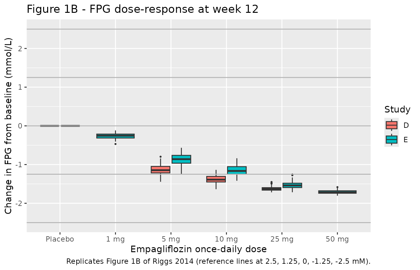
med12 <- chg |>
  dplyr::filter(week == 12) |>
  dplyr::group_by(study, arm) |>
  dplyr::summarise(dfpg = median(dfpg), dhba1c = median(dhba1c), .groups = "drop")
knitr::kable(med12, digits = 3,
caption = "Median change from baseline at week 12 by study and arm.")| study | arm | dfpg | dhba1c |
|---|---|---|---|
| D | Placebo | 0.000 | -0.149 |
| D | 5 mg | -1.146 | -0.494 |
| D | 10 mg | -1.390 | -0.713 |
| D | 25 mg | -1.628 | -0.838 |
| E | Placebo | 0.000 | -0.194 |
| E | 1 mg | -0.254 | -0.299 |
| E | 5 mg | -0.861 | -0.465 |
| E | 10 mg | -1.165 | -0.570 |
| E | 25 mg | -1.539 | -0.819 |
| E | 50 mg | -1.717 | -0.758 |
pbo <- med12[med12$arm == "Placebo", c("study", "dfpg", "dhba1c")]
names(pbo) <- c("study", "dfpg_pbo", "dhba1c_pbo")
drug <- merge(med12[med12$arm != "Placebo", ], pbo, by = "study")

stopifnot(
  # The FPG system starts at its own steady state, so a placebo arm does not
  # move. Asserted on the median, not on any subject's extreme.
  all(abs(med12$dfpg[med12$arm == "Placebo"]) < 0.05),
  # Every drug arm lowers FPG; the smallest effect is study E at 1 mg, whose
  # AUC50 is roughly twice the pooled estimate.
  all(drug$dfpg < -0.15),
  # Every drug arm lowers HbA1c beyond its own study's placebo drift.
  all(drug$dhba1c - drug$dhba1c_pbo < -0.05),
  # Monotone FPG dose-response within each study (arm is an ordered factor).
  all(diff(med12$dfpg[med12$study == "D"]) < 0),
  all(diff(med12$dfpg[med12$study == "E"]) < 0)
)
The HbA1c medians are not asserted to be monotone in dose:
HbA1c change depends on the subject-level kHbA1c,in and
kHbA1c,out draws as well as on the FPG change, and each arm
is an independent draw, so the study E 25 and 50 mg medians can cross.
The FPG medians, which depend only on clearance, are monotone.
Riggs 2014 reports that the 10 and 25 mg doses reach 80 % and 90 % of
the maximal response on the pooled studies A + B + D AUC50,
but only 65 % and 82 % on the study E AUC50 - the paper’s
central sensitivity analysis.
pct_of_max <- function(dose_mg, study, fpg_base) {
  full <- ss(0, fpg_base, study)$glucose - ss(maxdose, fpg_base, study)$glucose
  100 * (ss(0, fpg_base, study)$glucose - ss(dose_mg, fpg_base, study)$glucose) / full
}
pom <- tibble::tibble(
  `AUC50 source` = c("Studies A + B + D", "Studies A + B + D",
                     "Study E", "Study E"),
  Dose = c("10 mg", "25 mg", "10 mg", "25 mg"),
  `Model (pct of maximum)` = c(pct_of_max(10, "D", 9.30), pct_of_max(25, "D", 9.30),
                               pct_of_max(10, "E", 9.30), pct_of_max(25, "E", 9.30)),
  `Published (pct)` = c(80, 90, 65, 82)
)
knitr::kable(pom, digits = 1,
caption = "Fraction of the maximal FPG response achieved, by AUC50 estimate.")| AUC50 source | Dose | Model (pct of maximum) | Published (pct) |
|---|---|---|---|
| Studies A + B + D | 10 mg | 78.2 | 80 |
| Studies A + B + D | 25 mg | 90.0 | 90 |
| Study E | 10 mg | 65.1 | 65 |
| Study E | 25 mg | 82.3 | 82 |
PKNCA validation
Riggs 2014 states the typical steady-state dosing-interval AUC for
four dose levels (“The typical calculated steady-state AUC values for
once daily doses of 1, 3, 10 and 25 mg were 225, 674, 2250 and 5620 nmol
l-1 h”). Those values are the paper’s own Dose / (CL/F)
calculation; running non-compartmental analysis over the simulated
steady-state dosing interval therefore checks that the two-compartment
ODE, the absorption lag and the unit conversion in the packaged model
actually deliver that exposure, rather than re-stating the identity.
nca_doses <- c(1, 3, 10, 25)
tau <- 24
n_days <- 30
start_ss <- n_days * 24   # time of the final dose

# Hourly through the accumulation phase, then dense over the steady-state
# dosing interval that the NCA is computed on.
obs_times <- sort(unique(c(
  seq(0, start_ss, by = 1),
  seq(start_ss, start_ss + tau, by = 0.02)
)))

nca_sim <- dplyr::bind_rows(lapply(seq_along(nca_doses), function(i) {
  d <- nca_doses[i]
  ev <- rxode2::et(amt = d, ii = tau, until = start_ss, cmt = "depot") |>
    rxode2::et(obs_times, cmt = "glucose")
  ev <- as.data.frame(ev)
  ev$WT <- 70
  ev$DOSE_EMPA_MGD <- d
  ev$STUDY_EMPA_A <- 1
  ev$STUDY_EMPA_B <- 0
  ev$STUDY_EMPA_C <- 0
  ev$STUDY_EMPA_D <- 0
  ev$STUDY_EMPA_E <- 0
  s <- rxode2::rxSolve(mod0, ev, returnType = "data.frame",
                       omega = NA, sigma = NA)
  s$id <- i
  s$treatment <- paste0(d, " mg")
  s
}))

# rxSolve output carries no evid column, so the dose records are rebuilt from
# the known schedule rather than filtered out of the simulation.
dose_df <- tidyr::expand_grid(
  id = seq_along(nca_doses),
  time = seq(0, start_ss, by = tau)
) |>
  dplyr::mutate(amt = nca_doses[id], treatment = paste0(nca_doses[id], " mg"))
sim_nca <- nca_sim |>
  dplyr::filter(!is.na(Cc)) |>
  dplyr::select(id, time, Cc, treatment)

# Guarantee a time = 0 record per subject; empagliflozin is extravascular, so
# the pre-dose concentration is 0.
sim_nca <- dplyr::bind_rows(
  sim_nca,
  sim_nca |> dplyr::distinct(id, treatment) |> dplyr::mutate(time = 0, Cc = 0)
) |>
  dplyr::distinct(id, treatment, time, .keep_all = TRUE) |>
  dplyr::arrange(id, treatment, time)

conc_obj <- PKNCA::PKNCAconc(sim_nca, Cc ~ time | treatment + id)
dose_obj <- PKNCA::PKNCAdose(dose_df, amt ~ time | treatment + id)

intervals <- data.frame(
  start = start_ss, end = start_ss + tau,
  cmax = TRUE, tmax = TRUE, auclast = TRUE, cav = TRUE
)

nca_res <- PKNCA::pk.nca(PKNCA::PKNCAdata(conc_obj, dose_obj, intervals = intervals))
published <- tibble::tribble(
  ~treatment, ~auclast,
  "1 mg",     225,
  "3 mg",     674,
  "10 mg",    2250,
  "25 mg",    5620
)

cmp <- nlmixr2lib::ncaComparisonTable(
  simulated = nca_res,
  reference = published,
  by = "treatment",
  params = "auclast",
  units = c(auclast = "nmol*h/L"),
  tolerance_pct = 20
)
knitr::kable(
  cmp,
  caption = paste("Simulated steady-state AUC0-24 against the typical values",
                  "reported in Riggs 2014 Results. * differs by >20%."),
  align = c("l", "l", "r", "r", "r")
)| NCA parameter | treatment | Reference | Simulated | % diff |
|---|---|---|---|---|
| AUClast (nmol*h/L) | 1 mg | 225 | 225 | -0.1% |
| AUClast (nmol*h/L) | 3 mg | 674 | 674 | +0.0% |
| AUClast (nmol*h/L) | 10 mg | 2250 | 2250 | -0.1% |
| AUClast (nmol*h/L) | 25 mg | 5620 | 5620 | -0.0% |
auc_sim <- as.data.frame(nca_res)
auc_sim <- auc_sim[auc_sim$PPTESTCD == "auclast", ]
auc_sim <- auc_sim[match(published$treatment, auc_sim$treatment), ]
rel_err <- abs(auc_sim$PPORRES - published$auclast) / published$auclast
rel_err
#> [1] 0.0013594419 0.0001222366 0.0013594152 0.0004709451
stopifnot(
  # Deterministic typical-value NCA on a dense grid: the only error is
  # trapezoidal, so 1 pct is generous.
  all(rel_err < 0.01),
  # Dose proportionality of the linear PK model.
  max(abs(auc_sim$PPORRES / nca_doses - auc_sim$PPORRES[1] / nca_doses[1])) < 1
)
Riggs 2014 Table 1 also reports the observed mean steady-state AUC normalised to a 10 mg dose, by study (1970, 1830, 2480, 2280 and 2130 nmolh/L for studies A to E). Those are cohort means carrying the full covariate model of the companion population PK paper (age, sex, race, total protein, serum creatinine), of which only the allometric weight term is retained here, so they are not a target this model can reproduce; the qualitative ordering it can* reproduce is that the lightest cohort (study C, 67.9 kg) has the highest exposure.
wt_by_study <- c(A = 94.6, B = 93.2, C = 67.9, D = 81.4, E = 89.2)
auc_by_wt <- vapply(names(wt_by_study),
                    function(s) ss(10, 8, "A", wt = wt_by_study[[s]])$auc,
                    numeric(1))
tibble::tibble(Study = names(wt_by_study),
               `Mean weight (kg)` = as.numeric(wt_by_study),
               `Model AUC at 10 mg (nmol*h/L)` = auc_by_wt,
               `Table 1 observed mean` = c(1970, 1830, 2480, 2280, 2130)) |>
  knitr::kable(digits = 0,
caption = "Weight-driven exposure ordering against Riggs 2014 Table 1.")| Study | Mean weight (kg) | Model AUC at 10 mg (nmol*h/L) | Table 1 observed mean |
|---|---|---|---|
| A | 95 | 1793 | 1970 |
| B | 93 | 1813 | 1830 |
| C | 68 | 2299 | 2480 |
| D | 81 | 2007 | 2280 |
| E | 89 | 1873 | 2130 |
Assumptions and deviations
Errata and corrections to the published equations
-
Equation 3 (FPG turnover) is printed with a sign that
contradicts the rest of the paper. As typeset on p. 1412 it
reads
d(FPG)/dt = kFPGin - kFPGout * FPG * (1 - STIM), which reduces FPG removal asSTIMrises and therefore makes empagliflozin raise FPG. That contradicts the Figure 3 schematic (where theSTIMnode sits on thekFPG,outarrow leaving the FPG box), the narrative (“this STIM function directly affected the removal rate of FPG”; “stimulation (STIM) lowered FPG”), and every number the paper reports. The packaged model usesd(FPG)/dt = kFPGin - kFPGout * FPG / (1 - STIM), which keepsSTIMon the removal arm and gives a steady state ofFPG_base * (1 - STIM), i.e. a maximal proportional decrease equal toSTIMitself. That is exactly how Table 2 labels its calculated 0.158 (“FPG maximal decrease (proportional)”), and it reproduces all four published maximal FPG decreases and all four published maximal HbA1c decreases to the printed precision (see the “Maximal steady-state FPG and HbA1c decreases” table above, including the two-significant-figure 0.81 percentage-point value). The alternative readingkFPGout * FPG * (1 + STIM)- which the successor analysis (Baron 2016, same group, samekFPGoutof 0.0407 1/h) does use - reproduces none of the eight. -
Equation 2’s hyperbolic denominator is missing its
betafactor. As typeset the drug term is(beta + 1) * Emax_truncated * AUC / (C*50 + AUC), whose asymptote is(beta + 1) * Emax_truncated = 0.126and whose half-maximal exposure isC*50 = 498. Table 2’s own “Calculated parameters” block reports 0.158 and 626 instead, and both follow from(beta + 1) * Emax_truncated * AUC / (C*50 + beta * AUC):Emax = (beta + 1) / beta * Emax_truncated = 1.795 / 0.795 * 0.0701 = 0.1583andAUC50 = C*50 / beta = 498 / 0.795 = 626.4. The same identity reproduces the study C (106) and study E (1210)AUC50values. The packaged model uses the corrected form and exposesemax_fpgandauc50as named intermediates so both can be read straight out of a solve. -
Equation 1 labels UGE in mg but every reported value is in
g. Table 2 gives baseline UGE as “3.71 (g per 24 h)” and
Umaxas “121 (g 24 h-1)”, and the narrative works in g/day throughout. The model uses g. - One Results sentence appears to shift its own numbers by one dose level. Riggs 2014 states that the 72 and 75 g/day UGE increases predicted at 10 and 25 mg for a baseline FPG of 8 mmol/L “increase to 80 and 88 g day-1 … for an FPG of 10.5 mM”. The model reproduces 72.0 and 75.4 g at FPG 8 mmol/L exactly, and at 10.5 mmol/L it gives 79.4 g for 3 mg (the dose discussed in the preceding sentence) and 88.1 g for 10 mg - so the paper’s “80 and 88” match the 3 mg and 10 mg predictions rather than the 10 mg and 25 mg ones. No parameter was tuned; the discrepancy is recorded rather than resolved.
-
The reported HbA1c half-life is 4.3 weeks;
theta_26gives 4.15 weeks.log(2) / 0.167 week-1 = 4.15weeks. The packaged model uses thetheta_26point estimate.
Non-paper-derived parameter values
-
e_wt_cl,e_wt_q,e_wt_vc,e_wt_vpand the 70 kg reference weight are not printed in Riggs 2014, which says only that “weight was included allometrically on each of these parameters”. They are taken from the companion population PK publication whose model Riggs 2014 uses (Riggs 2013, J Clin Pharmacol 53:1028-1038, Table 3), where all four rows are flagged FIXED:(WT/70)^0.75on CL/F and Q/F,(WT/70)^1on V2/F and V3/F. Each is annotated inline in the model file.
Structural assumptions
-
Exposure driver. Riggs 2014 carried the individual
dosing-interval AUC as a data item generated by the companion population
PK model. The packaged model recomputes it as
DOSE_EMPA_MGD * 1e6 / 450.9 / cl, which is exact for a linear disposition model at steady state under once-daily dosing and reproduces the four typical AUC values the paper prints. Consequently the drug effect is driven by the dose level and the individual clearance, not by the simulated concentration profile; a simulation that changes the dose must updateDOSE_EMPA_MGDas well asamt. The PK ODEs are retained so thatCcis available and so the NCA check above can be run. -
Baseline FPG is a study-level fixed effect with no
IIV. Riggs 2014 Table 2 reports one baseline FPG theta per
study and no
omegafor it. This vignette evaluates the paper’s baseline-FPG-conditional predictions by overriding the study A theta throughrxSolve(params = ); that is a presentation device, not a model change. -
Study A has no baseline HbA1c. Table 1 footnotes
study A’s HbA1c as “Not included in the E-R analyses”, so no
thetaexists for it. The model gives a study A subject the study B baseline (the other short phase I cohort) purely so that the HbA1c state has a defined initial condition. HbA1c changes are unaffected because the drug enters HbA1c only through FPG. -
The HbA1c system is not at steady state at time
zero. The estimated baseline HbA1c thetas do not equal
HbA1c_limit + (kHbA1cin / kHbA1cout) * FPG_baselinefor any study (7.18 vs 7.31 for study B, 7.85 vs 7.68 for study D, and so on), so a placebo arm drifts by roughly 0.1 to 0.2 percentage points over 12 weeks. This is a property of the published parameter set, not of the transcription, and is visible in the study D and E placebo boxes above. -
No residual error is attached to
Cc. Riggs 2014 reports residual variance for UGE, FPG and HbA1c only; the PK residual belongs to the companion population PK paper.Ccis returned as a derived quantity. -
Residual errors are log-normal, not proportional.
Table 2 reports a variance and a CV% for each endpoint, and the two are
related by
CV = sqrt(exp(variance) - 1)for all three (0.380 -> 68.0 % against a printed 67.9 %; 0.01461 -> 12.13 % against 12.1 %; 0.001287 -> 3.589 % against 3.59 %), which is the exponential-error relationship. The model therefore uses~ lnorm(...)rather than~ prop(...). -
Model domain.
STIMmust stay below 1 for the FPG equation to be defined.STIMreaches 1 only at a baseline FPG of about 28 mmol/L, well above the highest baseline observed in the pooled cohort (21.0 mmol/L, study D).
Not modelled
-
Tolerability exposure-response. Riggs 2014
evaluated hypoglycaemia (n = 4), urinary tract infection (n = 17) and
genital / vulvovaginal events (n = 16) in studies D and E using
non-parametric generalised additive model smooths (Figure 6) rather than
a parametric model, and reported no increase in event probability with
exposure up to 50 mg. There are no coefficients to transcribe, so no
tolerability sub-model is carried; sex, which was screened in that
analysis, is recorded in
covariatesDataExcluded. -
Renal function. The influence of creatinine
clearance on the FPG and HbA1c responses was investigated graphically
only (Supplementary Figures S1 and S2) and none was found down to about
50 mL/min.
CRCLis recorded incovariatesDataExcluded. - Cohort demographics. The virtual cohorts above sample body weight from a normal distribution matched to the Table 1 study means and standard deviations, truncated to 45 to 150 kg. No other covariate distribution is needed because weight is the only covariate the retained model uses.