p-Furoylamphenmulin against Mycoplasma gallisepticum in chickens (Xia 2025)
Source:vignettes/articles/Xia_2025_pfuroylamphenmulin.Rmd
Xia_2025_pfuroylamphenmulin.RmdModel and source
Xia 2025 evaluated p-furoylamphenmulin – a semi-synthetic pleuromutilin made by adding a furoyl group to amphenmulin – against Mycoplasma gallisepticum in an intratracheally infected specific-pathogen-free chicken model. A single-dose plasma pharmacokinetic study at 5, 40 and 80 mg/kg intramuscular was combined with a three-day efficacy study spanning 0-80 mg/kg once daily, and the two were tied together with an inhibitory sigmoid Emax PK/PD-index model to recommend a dose.
The extraction is a single model file, because the authors’ structure is a single sequentially coupled chain: the compartmental PK supplies the exposure index that drives the exposure-response fit, and the paper’s dose recommendation is that chain inverted.
Model:
Xia_2025_pfuroylamphenmulinCitation: Xia X, Zhao H, Li Y, Long X, Liu X, Bai M, Tang Y, Shen X, Ding H. (2025). Pharmacokinetic/pharmacodynamic relationship of a novel pleuromutilin derivative p-furoylamphenmulin against Mycoplasma gallisepticum in vivo in chickens. Poultry Science 104(8):105249. doi:10.1016/j.psj.2025.105249.
Description: Preclinical (chicken, specific-pathogen-free, Mycoplasma gallisepticum-infected). Two-compartment first-order-absorption plasma PK model for the novel pleuromutilin derivative p-furoylamphenmulin after intramuscular injection in M. gallisepticum-infected chicks, coupled to the paper’s inhibitory sigmoid Emax PK/PD-index model for the reduction in lung mycoplasma load. PK from Xia 2025 Table 1 (mean of the 5, 40 and 80 mg/kg dose-group WinNonlin 5.2.1 fits): T1/2ka 0.0961 h, T1/2kel 4.2281 h, V1/F 6.3427 L/kg, V2/F 2.2405 L/kg, Cl/F 3.8692 L/h/kg. Xia 2025 reports no intercompartmental clearance, but the five reported quantities determine the two-compartment system exactly, so lq is DERIVED algebraically from them (see the ini() comment and the vignette). PD from Xia 2025 Table 2, AUC24h/MIC column: the 72 h reduction in lung load is E = E(0) + (Emax - E(0)) * Ce^N / (EC50^N + Ce^N) with E(0) = 1.07 log10 CFU/mL at zero exposure, a maximum of 4.29 log10 CFU/mL, EC50 = 7526.81 h and Hill N = 4.22. NOTE the paper’s Table 2 row labels are inverted relative to the usual convention: its ‘Emax’ row (1.07) is the zero-exposure effect and its ‘E0’ row (4.29) is the maximum effect, as Xia 2025 defines them in Materials and methods and confirms in Results. Substituting Table 2 into the equation at the paper’s own 3 log10 CFU/mL target of AUC24h/MIC = 8288.29 h returns E = 3.003, confirming the role assignment. The PK/PD index is formed from the closed form AUC24h = dose / (Cl/F), which is how Xia 2025 itself defines Cl/F (Dose/AUC24h reproduces every Table 1 AUC to nine decimal places) and how its dose-calculation formula (2) inverts it to the recommended 62.64 mg/kg. The lung mycoplasma density bact (linear CFU/mL) is integrated as d/dt(bact) = -ln(10) * (E / 72) * bact so that log10(bact) falls by exactly E across the paper’s 72 h treatment course, reproducing the endpoint model at the single time Xia 2025 actually counted bacteria. Xia 2025 reports neither between-subject variability nor a residual error magnitude for either endpoint, so no eta parameters are present and both residual SDs are FIXED at 0 for typical-value simulation. The companion Cmax/MIC parameterisation of Table 2 is not packaged as a separate file because a running Cmax is not an ODE quantity; it is reproduced in full in the vignette.
Population
368 one-day-old specific-pathogen-free chickens (35-45 g) were acclimatised for three days and then challenged intratracheally with 0.2 mL of a 10^9 CFU/mL M. gallisepticum S6 (ATCC 15302) suspension once daily for three consecutive days. 288 infected chicks entered the pharmacokinetic study (single intramuscular injection of 5, 40 or 80 mg/kg in 10% DMSO / 10% Tween 80 / 80% saline) and 80 entered the efficacy study (0, 5, 10, 20, 30, 40, 50, 60, 70 or 80 mg/kg once daily for three days, eight chicks per group), alongside tiamulin fumarate 40 mg/kg comparator arms.
Blood was drawn only once per chick (0.5 mL by cardiac puncture), so the plasma profile is a destructive-sampling naive-pooled design with eight different animals contributing at each of the twelve nominal times. There is consequently no individual-level PK and no hierarchical structure to estimate variance components from, which is why the packaged model carries no between-subject variability.
Lungs were collected, homogenised and plated 24 h after the last of the three daily doses, i.e. 72 h after the first dose – a single count per animal, which is why the exposure-response is an endpoint model rather than a time-kill model.
The same information is available programmatically via the model’s
population metadata
(readModelDb("Xia_2025_pfuroylamphenmulin")()$population).
Source trace
The per-parameter origin is recorded as an in-file comment next to
each ini() entry in
inst/modeldb/specificDrugs/Xia_2025_pfuroylamphenmulin.R.
The table below collects them in one place. Supplementary files
mmc1-mmc6 accompany the article at the same
DOI; mmc5.xlsx carries the individual plasma concentrations
and the full-precision compartmental parameter summary that Table 1
rounds, and mmc4.xlsx carries the individual lung counts
behind Figure 2.
| Equation / parameter | Value | Source location |
|---|---|---|
First-order absorption two-compartment PK (depot,
central, peripheral1) |
n/a | Materials and methods, “Pharmacokinetic data analysis”: WinNonlin 5.2.1, “the first-order absorption two-compartment model was used” |
lka |
log(log(2) / 0.0961057) = log(7.2123)
|
Table 1, T1/2ka = 0.10 +/- 0.01 h; full precision from
mmc5.xlsx
|
lcl |
log(3.86921107) |
Table 1, Cl/F = 3.87 +/- 0.28 L/h/kg; full precision from
mmc5.xlsx
|
lvc |
log(6.3427335) |
Table 1, V1/F = 6.34 +/- 0.76 L/kg; full precision from
mmc5.xlsx
|
lvp |
log(2.240488147) |
Table 1, V2/F = 2.24 +/- 0.48 L/kg; full precision from
mmc5.xlsx
|
lq |
log(0.42209916) |
DERIVED from Table 1 Cl/F, V1/F, V2/F and T1/2kel = 4.2281 h – see Assumptions and deviations |
tau |
24 h (FIXED) | Abstract and Dose calculation: “intramuscular injection once every 24 h for 3 consecutive days”; the index is AUC24h/MIC |
d/dt(auc_0_24) <- Cc * (t < tau) |
n/a | Materials and methods, “PK/PD fitting analysis”: the index is AUC24h/MIC |
auc24 <- podo(depot) / cl |
n/a | Table 1, where Dose / (Cl/F) reproduces every reported AUC24h; Dose calculation formula (2) inverts the same relation |
kill72 <- e0 + (emax - e0) * aucmic^hill / (ec50^hill + aucmic^hill) |
n/a | Materials and methods, “PK/PD fitting analysis”: Inhibitory Sigmoid Emax model in WinNonlin |
e0 |
1.07 log10 CFU/mL | Table 2, AUC24h/MIC column, row labelled “Emax”; Results: at 0 mg/kg the load “naturally decreased by 1.07-1.09 Log10CFU/mL” |
lemax |
log(4.29) |
Table 2, AUC24h/MIC column, row labelled “E0”; Materials and methods: “E0 = maximum antimicrobial effect reached after 72 h” |
lec50 |
log(7526.81) |
Table 2, AUC24h/MIC column, EC50 = 7526.81 |
lhill |
log(4.22) |
Table 2, AUC24h/MIC column, Hill’s slope = 4.22 |
mic |
0.001953125 ug/mL (FIXED) | Results, “Susceptibility changes”; supplementary
mmc3.xlsx
|
log10_cfu0 |
6.13035274875 (FIXED) | Supplementary mmc4.xlsx, mean 0 h count of the efficacy
cohort (n = 8) |
d/dt(bact) <- -log(10) * (kill72 / 72) * bact |
n/a | Materials and methods: E is “the change in mycoplasma load in the lungs during 72 h of treatment”; lungs sampled once, 24 h after the last of three daily doses |
propSd |
0 (FIXED) | Not reported; Results gives bioanalytical recovery and precision only |
addSd_log10cfu |
0 (FIXED) | Not reported; Table 2 gives R^2 = 0.83 only |
Published reference values used for validation below:
| Quantity | 5 mg/kg | 40 mg/kg | 80 mg/kg | Mean +/- SEM | Source |
|---|---|---|---|---|---|
| T1/2kel (h) | 4.21 | 3.61 | 4.87 | 4.23 +/- 0.37 | Table 1 |
| T1/2ka (h) | 0.09 | 0.12 | 0.07 | 0.10 +/- 0.01 | Table 1 |
| Cmax (ug/mL) | 0.56 | 5.79 | 9.53 | – | Table 1 |
| Tmax (h) | 0.38 | 0.39 | 0.30 | 0.36 +/- 0.03 | Table 1 |
| AUC24h (ug*h/mL) | 1.49 | 10.15 | 18.56 | – | Table 1 |
| V1/F (L/kg) | 7.39 | 4.86 | 6.78 | 6.34 +/- 0.76 | Table 1 |
| V2/F (L/kg) | 1.49 | 2.11 | 3.11 | 2.24 +/- 0.48 | Table 1 |
| Cl/F (L/h/kg) | 3.35 | 3.94 | 4.31 | 3.87 +/- 0.28 | Table 1 |
The derivation of lq
Xia 2025 reports five quantities for the first-order-absorption
two-compartment model – T1/2ka, T1/2kel,
V1/F, V2/F and Cl/F – which is
exactly the number a two-compartment model with first-order input needs.
No intercompartmental clearance is printed, but it is not free: it is
pinned by the other four disposition quantities.
The key step is establishing what T1/2kel is. In a
two-compartment model alpha > k10 > beta, so a
reported half-life can only be the terminal (beta) half-life if
ln(2)/T1/2kel < k10.
tab1 <- tibble::tribble(
  ~dose, ~t12kel,  ~t12ka,   ~cmax,    ~tmax,  ~auc24h,    ~v1f,     ~v2f,     ~clf,
      5, 4.205003, 0.089020, 0.5616932, 0.379236,  1.490474995, 7.392317373, 1.488610296, 3.354635278,
     40, 3.607271, 0.124374, 5.7915220, 0.389907, 10.148484359, 4.855186731, 2.113410516, 3.941475257,
     80, 4.871964, 0.074923, 9.5313792, 0.300782, 18.554929668, 6.780696396, 3.119443629, 4.311522675
)
tab1_mean <- list(
  t12kel = 4.22807933333333, t12ka = 0.0961056666666667, tmax = 0.356641666666667,
  v1f = 6.3427335, v2f = 2.240488147, vdf = 8.583221647, clf = 3.86921107
)

# (a) Cl/F is defined so that Dose / (Cl/F) IS the reported AUC24h.
tab1 |>
  transmute(
    dose,
    reported_auc24h = auc24h,
    dose_over_cl = dose / clf,
    abs_diff = abs(dose / clf - auc24h)
  ) |>
  dplyr::rename(
    "Dose (mg/kg)" = dose, "Reported AUC24h" = reported_auc24h,
    "Dose / (Cl/F)" = dose_over_cl, "|difference|" = abs_diff
  ) |>
knitr::kable(digits = 10, caption = "Xia 2025 Table 1: Cl/F is Dose divided by AUC24h.")| Dose (mg/kg) | Reported AUC24h | Dose / (Cl/F) | |difference| |
|---|---|---|---|
| 5 | 1.490475 | 1.490475 | 2e-10 |
| 40 | 10.148484 | 10.148484 | 7e-10 |
| 80 | 18.554930 | 18.554930 | 8e-10 |
stopifnot(max(abs(tab1$dose / tab1$clf - tab1$auc24h)) < 1e-8)

# (b) ln(2)/k10 is nothing like the reported T1/2kel, so T1/2kel is terminal.
k10_halflife <- log(2) / (tab1$clf / tab1$v1f)
round(rbind("ln(2)/k10 (h)" = k10_halflife, "reported T1/2kel (h)" = tab1$t12kel), 3)
#>                       [,1]  [,2]  [,3]
#> ln(2)/k10 (h)        1.527 0.854 1.090
#> reported T1/2kel (h) 4.205 3.607 4.872
stopifnot(all(log(2) / tab1$t12kel < tab1$clf / tab1$v1f))
The reported T1/2kel is therefore the terminal
half-life, and Q/F follows from the smaller root of the
two-compartment characteristic equation
beta^2 - (k10 + k12 + k21) beta + k10 k21 = 0 with
k12 = Q/V1, k21 = Q/V2:
derive_q <- function(cl, v1, v2, t12_terminal) {
  k10 <- cl / v1
  beta <- log(2) / t12_terminal
  beta * (k10 - beta) / (k10 / v2 - beta * (1 / v1 + 1 / v2))
}
terminal_t12 <- function(cl, v1, v2, q) {
  k10 <- cl / v1; k12 <- q / v1; k21 <- q / v2
  s <- k10 + k12 + k21
  log(2) / ((s - sqrt(s^2 - 4 * k10 * k21)) / 2)
}

q_per_dose <- derive_q(tab1$clf, tab1$v1f, tab1$v2f, tab1$t12kel)
q_mean_col <- derive_q(tab1_mean$clf, tab1_mean$v1f, tab1_mean$v2f, tab1_mean$t12kel)

c(`Q/F 5 mg/kg` = q_per_dose[1], `Q/F 40 mg/kg` = q_per_dose[2],
  `Q/F 80 mg/kg` = q_per_dose[3], `mean of the three` = mean(q_per_dose),
  `Q/F from the mean column (packaged)` = q_mean_col) |>
  round(5)
#>                         Q/F 5 mg/kg                        Q/F 40 mg/kg
#>                             0.27723                             0.46947
#>                        Q/F 80 mg/kg                   mean of the three
#>                             0.51166                             0.41945
#> Q/F from the mean column (packaged)
#>                             0.42210

# Round-trip: the derived Q must return the reported terminal half-life.
round(terminal_t12(tab1_mean$clf, tab1_mean$v1f, tab1_mean$v2f, q_mean_col), 6)
#> [1] 4.228079
stopifnot(
  abs(terminal_t12(tab1_mean$clf, tab1_mean$v1f, tab1_mean$v2f, q_mean_col) -
        tab1_mean$t12kel) < 1e-6,
  all(q_per_dose > 0),
  # the packaged value agrees with the mean of the per-dose derivations to <1%
  abs(q_mean_col / mean(q_per_dose) - 1) < 0.01
)

stopifnot(abs(exp(mod$theta[["lq"]]) - q_mean_col) < 1e-6)
The third, independent check is empirical: the log-linear slope of
the observed mean concentrations between 12 and 24 h (supplementary
mmc5.xlsx) recovers the reported T1/2kel per
dose group, confirming it is the terminal phase and not a
micro-constant.
obs_12_24 <- tibble::tribble(
  ~dose, ~c12,                 ~c24,
      5, 0.00620571428571429,  0.0008267,
     40, 0.037585,             0.0033025,
     80, 0.0990875,            0.0141125
) |>
  mutate(
    observed_t12 = log(2) / (log(c12 / c24) / 12),
    reported_t12 = tab1$t12kel
  )

obs_12_24 |>
  select(dose, observed_t12, reported_t12) |>
  mutate(across(where(is.numeric), \(x) round(x, 3))) |>
  dplyr::rename(
    "Dose (mg/kg)" = dose,
    "Observed 12-24 h t1/2 (h)" = observed_t12,
    "Reported T1/2kel (h)" = reported_t12
  ) |>
knitr::kable(caption = "Observed terminal slope versus the reported T1/2kel.")| Dose (mg/kg) | Observed 12-24 h t1/2 (h) | Reported T1/2kel (h) |
|---|---|---|
| 5 | 4.126 | 4.205 |
| 40 | 3.420 | 3.607 |
| 80 | 4.268 | 4.872 |
Virtual cohort
The source study has no virtual population to sample: each arm is a dose level given to eight chicks, individual PK is unavailable by design (one blood draw per animal), and the paper reports no variance components. Arms are therefore enumerated deterministically and every simulation below is a typical-value solve.
# Observation rows sit on the ODE state `central`; `dvid = 1L` selects the Cc
# endpoint of this two-endpoint model. rxode2 returns every algebraic observable
# (Cc, auc24, aucmic, kill72, log10cfu) as a column at these rows.
#
# The untreated control arm uses explicit amt = 0 dose records: podo(depot) is
# NA until a dose has been seen, and 0 afterwards.
make_events <- function(dose, n_doses = 3L, tmax = 72, times = NULL) {
  if (is.null(times)) {
    times <- sort(unique(c(seq(0, tmax, by = 0.25), 0.083, 0.25, 0.5, 1, 2, 3, 4, 6, 8, 10, 12, 24)))
  }
  doses <- data.frame(
    time = seq(0, by = 24, length.out = n_doses),
    amt = dose, cmt = "depot", evid = 1L, dvid = NA_integer_
  )
  obs <- data.frame(
    time = times, amt = NA_real_, cmt = "central", evid = 0L, dvid = 1L
  )
  bind_rows(doses, obs) |> arrange(time, desc(evid))
}

# `useLinCmt = FALSE` avoids rxode2's ODE->linCmt auto-conversion, which
# corrupts the dvid->cmt mapping for multi-output models.
solve_arm <- function(dose, ...) {
  rxode2::rxSolve(
    mod, make_events(dose, ...),
    useLinCmt = FALSE, returnType = "data.frame"
  ) |>
    mutate(dose_mgkg = dose)
}
Internal consistency
The model carries the exposure index twice: auc_0_24
integrates Cc over the first dosing interval, while
auc24 is the closed form podo(depot) / cl that
Xia 2025’s own Table 1 defines. They must agree, and the closed form
must equal Dose / (Cl/F) exactly.
consistency <- bind_rows(lapply(c(5, 40, 80), function(d) {
  s <- solve_arm(d, n_doses = 1L, tmax = 24,
                 times = sort(unique(c(seq(0, 24, by = 0.002), 24))))
  tibble::tibble(
    dose = d,
    integrated_auc0_24 = max(s$auc_0_24),
    closed_form_auc24 = unique(s$auc24),
    dose_over_cl = d / exp(mod$theta[["lcl"]])
  )
})) |>
  mutate(pct_gap = 100 * (integrated_auc0_24 / closed_form_auc24 - 1))

consistency |>
  mutate(across(where(is.numeric), \(x) signif(x, 6))) |>
  dplyr::rename(
    "Dose (mg/kg)" = dose,
    "Integrated AUC0-24 (ug*h/mL)" = integrated_auc0_24,
    "Closed-form AUC24h (ug*h/mL)" = closed_form_auc24,
    "Dose / (Cl/F)" = dose_over_cl,
    "Integrated vs closed form (%)" = pct_gap
  ) |>
knitr::kable(caption = "Integrated versus closed-form exposure index.")| Dose (mg/kg) | Integrated AUC0-24 (ug*h/mL) | Closed-form AUC24h (ug*h/mL) | Dose / (Cl/F) | Integrated vs closed form (%) |
|---|---|---|---|---|
| 5 | 1.28787 | 1.29225 | 1.29225 | -0.339057 |
| 40 | 10.30300 | 10.33800 | 10.33800 | -0.339051 |
| 80 | 20.60590 | 20.67600 | 20.67600 | -0.339065 |
# The closed form must BE Dose/(Cl/F) to solver precision.
stopifnot(max(abs(consistency$closed_form_auc24 - consistency$dose_over_cl)) < 1e-9)
# The 0-24 h integral falls short of AUC-infinity only by the extrapolated tail,
# which for a 4.23 h terminal half-life is a few tenths of a percent.
stopifnot(all(consistency$pct_gap < 0), all(consistency$pct_gap > -1))
The -0.34% gap is the tail of the profile beyond 24 h.
It is the price of the paper’s own convention – Xia 2025 labels
Dose / (Cl/F) as “AUC24h” – and is far smaller than the
between-dose-group spread discussed below.
Replicate Figure 1: plasma concentration-time curves
Figure 1 shows the mean concentration-time curves after single
intramuscular doses of 5, 40 and 80 mg/kg (n = 8 per time point). The
observed means and standard errors below are transcribed from
supplementary mmc5.xlsx.
observed_pk <- tibble::tribble(
  ~dose, ~time,  ~conc,                ~sem,
      5, 0.083,  0.6822,               0.0864282361268584,
      5, 0.25,   0.63125,              0.108176071753415,
      5, 0.5,    0.621,                0.0273691693072959,
      5, 1,      0.338625,             0.0149582006891585,
      5, 2,      0.250285714285714,    0.0458796117628539,
      5, 3,      0.153125,             0.00679925810028459,
      5, 4,      0.1152,               0.00913689537769023,
      5, 6,      0.0489125,            0.00857076504128174,
      5, 8,      0.02704625,           0.00490138061362743,
      5, 10,     0.014535,             0.0018475302046632,
      5, 12,     0.00620571428571429,  0.00203780677753928,
      5, 24,     0.0008267,            0.00037544585495115,
     40, 0.083,  4.2105,               0.202920022950634,
     40, 0.25,   4.373,                0.468060893474343,
     40, 0.5,    5.21,                 0.177562866130763,
     40, 1,      4.4075,               0.420058796904841,
     40, 2,      2.4505,               0.235955125878993,
     40, 3,      0.710375,             0.0451714738919534,
     40, 4,      0.346,                0.0474051684945851,
     40, 6,      0.17225,              0.0340329409753047,
     40, 8,      0.0643875,            0.0097132170171076,
     40, 10,     0.0619375,            0.00350244493685686,
     40, 12,     0.037585,             0.00525831416493374,
     40, 24,     0.0033025,            0.00137677990857895,
     80, 0.083,  7.345,                1.03827267269111,
     80, 0.25,   7.578,                0.538757830569543,
     80, 0.5,    8.099,                0.524708218237254,
     80, 1,      7.676,                0.66288201923764,
     80, 2,      4.772,                0.360111093969625,
     80, 3,      2.004,                0.203067898567379,
     80, 4,      0.71925,              0.0937479047384908,
     80, 6,      0.437875,             0.0796742110768239,
     80, 8,      0.1507,               0.021850237004272,
     80, 10,     0.1119125,            0.00470795062709273,
     80, 12,     0.0990875,            0.0128373400323877,
     80, 24,     0.0141125,            0.000607229510622984
)

pk_sim <- bind_rows(lapply(c(5, 40, 80), function(d) {
  solve_arm(d, n_doses = 1L, tmax = 24,
            times = sort(unique(c(seq(0, 24, by = 0.01), 0.083))))
}))

lloq <- 0.001  # Results: LOQ 1 ng/mL, LOD 0.5 ng/mL

ggplot(pk_sim, aes(time, Cc, colour = factor(dose_mgkg))) +
  geom_line() +
  geom_pointrange(
    data = observed_pk,
    aes(time, conc, ymin = pmax(conc - sem, 1e-5), ymax = conc + sem,
        colour = factor(dose)),
    inherit.aes = FALSE, size = 0.25
  ) +
  geom_hline(yintercept = lloq, linetype = "dotted") +
  scale_y_log10() +
  scale_x_continuous(breaks = seq(0, 24, by = 4)) +
  labs(
    x = "Time (h)", y = "p-furoylamphenmulin plasma concentration (ug/mL)",
    colour = "Dose (mg/kg)",
    title = "Figure 1 -- single-dose intramuscular plasma profiles",
    caption = paste(
      "Replicates Figure 1 of Xia 2025. Lines are the packaged mean-parameter",
      "model; points are observed means +/- SEM (n = 8) from supplementary",
      "mmc5.xlsx. Dotted line = the 1 ng/mL limit of quantitation."
    )
  ) +
  theme(legend.position = "bottom")
#> Warning in scale_y_log10(): log-10 transformation introduced infinite values.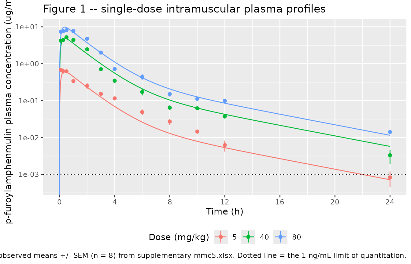
The packaged model uses the Table 1 mean parameter
column – the column the paper’s own dose calculation uses – so it is a
compromise across three dose groups whose Cl/F rises from
3.35 to 4.31 L/h/kg. It therefore sits above the observed 5 mg/kg
profile and slightly below the 40 mg/kg peak. The per-dose-group
parameter sets are recorded in the model’s
population$notes.
PKNCA validation
# Truncate at the published LOQ: below 1 ng/mL the paper's own data are
# unquantifiable, and a terminal slope fitted into that region is not comparable
# with the published one.
sim_nca <- pk_sim |>
  filter(!is.na(Cc)) |>
  mutate(treatment = paste0(dose_mgkg, " mg/kg"), id = 1L) |>
  filter(Cc >= lloq | time == 0) |>
  select(id, treatment, time, Cc)

# Guarantee a time = 0 record per arm so PKNCA can anchor AUC from t = 0.
sim_nca <- bind_rows(
  sim_nca,
  sim_nca |> distinct(id, treatment) |> mutate(time = 0, Cc = 0)
) |>
  distinct(treatment, id, time, .keep_all = TRUE) |>
  arrange(treatment, id, time)

conc_obj <- PKNCA::PKNCAconc(sim_nca, Cc ~ time | treatment + id)

dose_df <- pk_sim |>
  distinct(dose_mgkg) |>
  mutate(treatment = paste0(dose_mgkg, " mg/kg"), id = 1L, time = 0, amt = dose_mgkg) |>
  select(id, treatment, time, amt)

dose_obj <- PKNCA::PKNCAdose(dose_df, amt ~ time | treatment + id)

intervals <- data.frame(
  start = 0, end = 24,
  cmax = TRUE, tmax = TRUE, auclast = TRUE, aucinf.obs = TRUE, half.life = TRUE
)

nca_res <- PKNCA::pk.nca(PKNCA::PKNCAdata(conc_obj, dose_obj, intervals = intervals))
nca_tidy <- as.data.frame(nca_res) |>
  filter(PPTESTCD %in% c("cmax", "tmax", "auclast", "aucinf.obs", "half.life")) |>
  select(treatment, PPTESTCD, PPORRES) |>
  tidyr::pivot_wider(names_from = PPTESTCD, values_from = PPORRES)

nca_tidy |>
  mutate(across(where(is.numeric), \(x) signif(x, 4))) |>
  dplyr::rename(
    "Treatment" = treatment,
    "Cmax (ug/mL)" = cmax,
    "Tmax (h)" = tmax,
    "AUC0-24 (ug*h/mL)" = auclast,
    "AUC0-inf (ug*h/mL)" = aucinf.obs,
    "t1/2 (h)" = half.life
  ) |>
knitr::kable(caption = "PKNCA results for the simulated single-dose profiles.")| Treatment | AUC0-24 (ug*h/mL) | Cmax (ug/mL) | Tmax (h) | t1/2 (h) | AUC0-inf (ug*h/mL) |
|---|---|---|---|---|---|
| 40 mg/kg | 10.300 | 4.9380 | 0.36 | 4.172 | 10.340 |
| 5 mg/kg | 1.286 | 0.6173 | 0.36 | 4.162 | 1.292 |
| 80 mg/kg | 20.610 | 9.8770 | 0.36 | 4.172 | 20.670 |
Comparison against published NCA
published_pk <- tibble::tribble(
  ~treatment,   ~cmax,     ~tmax,    ~aucinf.obs,  ~half.life,
  "5 mg/kg",    0.561693,  0.379236,  1.490475,    4.205003,
  "40 mg/kg",   5.791522,  0.389907, 10.148484,    3.607271,
  "80 mg/kg",   9.531379,  0.300782, 18.554930,    4.871964
)

cmp_pk <- nlmixr2lib::ncaComparisonTable(
  simulated = nca_tidy,
  reference = published_pk,
  by = "treatment",
  params = c("cmax", "tmax", "aucinf.obs", "half.life"),
  units = c(cmax = "ug/mL", tmax = "h", aucinf.obs = "ug*h/mL", half.life = "h"),
  tolerance_pct = 20
)

knitr::kable(
  cmp_pk,
  caption = paste(
    "Simulated versus published PK. Reference values are the per-dose-group",
    "WinNonlin fits of Xia 2025 Table 1 at the full precision of supplementary",
    "mmc5.xlsx; the simulation uses the single Table 1 MEAN parameter column.",
    "* differs from reference by >20%."
  )
)| NCA parameter | treatment | Reference | Simulated | % diff |
|---|---|---|---|---|
| Cmax (ug/mL) | 5 mg/kg | 0.562 | 0.617 | +9.9% |
| Cmax (ug/mL) | 40 mg/kg | 5.79 | 4.94 | -14.7% |
| Cmax (ug/mL) | 80 mg/kg | 9.53 | 9.88 | +3.6% |
| Tmax (h) | 5 mg/kg | 0.379 | 0.36 | -5.1% |
| Tmax (h) | 40 mg/kg | 0.39 | 0.36 | -7.7% |
| Tmax (h) | 80 mg/kg | 0.301 | 0.36 | +19.7% |
| AUC0-∞ (obs) (ug*h/mL) | 5 mg/kg | 1.49 | 1.29 | -13.3% |
| AUC0-∞ (obs) (ug*h/mL) | 40 mg/kg | 10.1 | 10.3 | +1.9% |
| AUC0-∞ (obs) (ug*h/mL) | 80 mg/kg | 18.6 | 20.7 | +11.4% |
| t½ (h) | 5 mg/kg | 4.21 | 4.16 | -1.0% |
| t½ (h) | 40 mg/kg | 3.61 | 4.17 | +15.7% |
| t½ (h) | 80 mg/kg | 4.87 | 4.17 | -14.4% |
chk <- nca_tidy |> left_join(published_pk, by = "treatment", suffix = c("_sim", "_ref"))

# The mean-parameter model must reproduce every per-dose-group value to within
# 20%, which is the spread the dose groups themselves show.
stopifnot(max(abs(chk$cmax_sim / chk$cmax_ref - 1)) < 0.20)
stopifnot(max(abs(chk$aucinf.obs_sim / chk$aucinf.obs_ref - 1)) < 0.20)
stopifnot(max(abs(chk$half.life_sim / chk$half.life_ref - 1)) < 0.20)

# Against the parameter set actually packaged -- the Table 1 MEAN column -- the
# agreement is far tighter: the model IS that column.
stopifnot(max(abs(chk$tmax_sim / tab1_mean$tmax - 1)) < 0.03)
# PKNCA's automatic lambda-z window reaches back to about 12 h, where a trace of
# the distribution phase survives, so the NCA half-life sits ~1.2% below the
# model's exact terminal half-life. The exact value is asserted analytically in
# "The derivation of lq" above (terminal_t12() round-trips to 4.228079 h); this
# is the looser NCA cross-check, tightened to the accuracy actually achieved.
stopifnot(max(abs(chk$half.life_sim / tab1_mean$t12kel - 1)) < 0.02)
# AUC must be Dose/(Cl/F) of the mean column, to the accuracy of the NCA grid.
auc_ratio <- chk$aucinf.obs_sim / (c(5, 40, 80)[match(chk$treatment, published_pk$treatment)] /
                                     tab1_mean$clf)
stopifnot(max(abs(auc_ratio - 1)) < 0.01)
Tmax is flagged only for the 80 mg/kg group: the model
is linear, so it predicts one Tmax (0.36 h) for every dose,
which is within 2% of the Table 1 mean of 0.357 h but 20% above the
0.301 h fitted to that one dose group.
The paper’s %T>MIC statement
Xia 2025 explicitly declined to use %T>MIC as the index because it could not discriminate: “The %T>MIC within 24 h at 5 mg/kg was 89.53% and 100% at higher doses.” The model reproduces the saturation at 40 and 80 mg/kg immediately, but gives 74.6% rather than 89.53% at 5 mg/kg.
That gap is fully explained, and it is a property of the paper’s arithmetic rather than of the model. Only the 5 mg/kg profile crosses the MIC inside 24 h, and it does so inside the 12 h gap between the last two samples. Interpolating that gap linearly on the observed means reproduces 89.53% to four significant figures; interpolating it log-linearly, which is what a first-order decay requires, gives 78.7% – and that is what the model returns when it is run with the 5 mg/kg group’s own parameters.
mic_value <- mod$theta[["mic"]]

t_above_model <- bind_rows(lapply(c(5, 40, 80), function(d) {
  s <- solve_arm(d, n_doses = 1L, tmax = 24, times = seq(0, 24, by = 0.001))
  tibble::tibble(dose = d, pct_model_mean_params = 100 * mean(s$Cc > mic_value))
}))

# The same quantity read straight off the observed 5 mg/kg means, both ways.
c12 <- observed_pk$conc[observed_pk$dose == 5 & observed_pk$time == 12]
c24 <- observed_pk$conc[observed_pk$dose == 5 & observed_pk$time == 24]
t_linear <- 12 + 12 * (c12 - mic_value) / (c12 - c24)
t_loglinear <- 12 + log(c12 / mic_value) / (log(c12 / c24) / 12)

tibble::tibble(
  method = c("Xia 2025 reported",
             "Observed means, LINEAR interpolation 12-24 h",
             "Observed means, log-linear interpolation 12-24 h",
             "Packaged mean-parameter model"),
  pct = c(89.53, 100 * t_linear / 24, 100 * t_loglinear / 24,
          t_above_model$pct_model_mean_params[1])
) |>
  mutate(pct = round(pct, 2)) |>
  dplyr::rename("Method" = method, "%T>MIC over 0-24 h at 5 mg/kg" = pct) |>
knitr::kable(caption = "Where the reported 89.53% comes from.")| Method | %T>MIC over 0-24 h at 5 mg/kg |
|---|---|
| Xia 2025 reported | 89.53 |
| Observed means, LINEAR interpolation 12-24 h | 89.53 |
| Observed means, log-linear interpolation 12-24 h | 78.67 |
| Packaged mean-parameter model | 74.61 |
t_above_model |>
  mutate(pct_model_mean_params = round(pct_model_mean_params, 2)) |>
  dplyr::rename("Dose (mg/kg)" = dose, "Model %T>MIC over 0-24 h" = pct_model_mean_params) |>
knitr::kable(caption = "Model %T>MIC across the three studied dose levels.")| Dose (mg/kg) | Model %T>MIC over 0-24 h |
|---|---|
| 5 | 74.61 |
| 40 | 100.00 |
| 80 | 100.00 |
# Linear interpolation of the 12-24 h gap reproduces the paper's number exactly.
stopifnot(abs(100 * t_linear / 24 - 89.53) < 0.01)
# Log-linear interpolation of the SAME observed data agrees with the model
# instead, to better than 5 percentage points.
stopifnot(abs(100 * t_loglinear / 24 - t_above_model$pct_model_mean_params[1]) < 5)
# The paper's actual point -- %T>MIC saturates and so cannot discriminate the
# observed effects -- holds in the model at 40 and 80 mg/kg.
stopifnot(all(t_above_model$pct_model_mean_params[2:3] > 99.9))
Replicate Figure 2: lung mycoplasma load after three daily doses
Figure 2 shows the M. gallisepticum lung load at 72 h for
each dose group against the 0 h baseline. The individual counts are in
supplementary mmc4.xlsx.
observed_pd <- tibble::tribble(
  ~dose, ~count72, ~count_sem, ~reduction, ~reduction_sem,
      0, 5.70458,  0.09958,    0.42577,    0.09958,
      5, 5.02260,  0.12893,    1.10775,    0.12893,
     10, 4.85267,  0.12717,    1.27768,    0.12717,
     20, 4.64096,  0.20956,    1.48939,    0.20956,
     30, 4.85953,  0.20728,    1.87826,    0.63341,
     40, 4.16339,  0.15869,    1.96696,    0.15869,
     50, 4.60489,  0.12837,    1.52546,    0.12837,
     60, 3.60697,  0.27972,    2.52338,    0.27972,
     70, 2.74510,  0.14447,    3.38526,    0.14447,
     80, 2.85139,  0.23070,    3.27896,    0.23070
)
baseline_0h <- 6.13035274875

dose_ladder <- observed_pd$dose

pd_sim <- bind_rows(lapply(dose_ladder, function(d) {
  solve_arm(d, n_doses = 3L, tmax = 72, times = seq(0, 72, by = 1))
}))

pd_endpoints <- pd_sim |>
  group_by(dose_mgkg) |>
  summarise(
    aucmic = first(aucmic),
    count72 = last(log10cfu),
    reduction = first(log10cfu) - last(log10cfu),
    .groups = "drop"
  )

ggplot(pd_sim, aes(time, log10cfu, colour = factor(dose_mgkg))) +
  geom_line() +
  geom_pointrange(
    data = observed_pd,
    aes(x = 72, y = count72, ymin = count72 - count_sem, ymax = count72 + count_sem,
        colour = factor(dose)),
    inherit.aes = FALSE, size = 0.25
  ) +
  geom_hline(yintercept = baseline_0h - 3, linetype = "dashed") +
  scale_x_continuous(breaks = seq(0, 72, by = 24)) +
  labs(
    x = "Time (h)", y = "M. gallisepticum lung load (log10 CFU/mL)",
    colour = "Dose (mg/kg)",
    title = "Figure 2 -- lung load over the three-day course",
    caption = paste(
      "Replicates Figure 2 of Xia 2025. Lines are the packaged model; points at",
      "72 h are observed means +/- SEM (n = 8) from supplementary mmc4.xlsx.",
      "Dashed line = a 3 log10 CFU/mL reduction from the 0 h baseline."
    )
  ) +
  theme(legend.position = "bottom")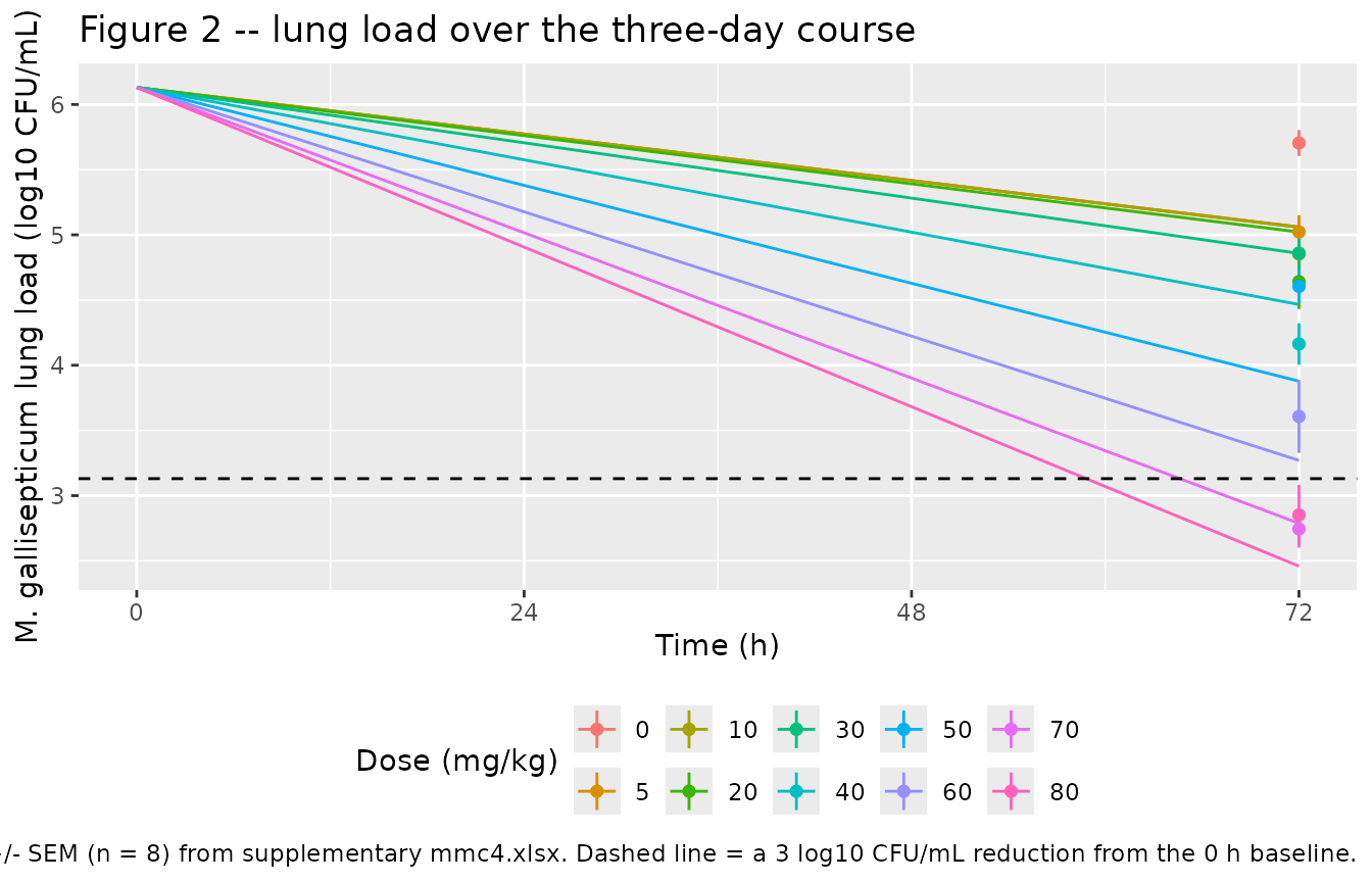
pd_cmp <- pd_endpoints |>
  left_join(observed_pd, by = c("dose_mgkg" = "dose"), suffix = c("_model", "_obs")) |>
  mutate(residual = reduction_model - reduction_obs)

pd_cmp |>
  select(dose_mgkg, aucmic, reduction_model, reduction_obs, reduction_sem, residual) |>
  mutate(aucmic = signif(aucmic, 5), across(where(is.numeric), \(x) round(x, 3))) |>
  dplyr::rename(
    "Dose (mg/kg)" = dose_mgkg,
    "Model AUC24h/MIC (h)" = aucmic,
    "Model reduction (log10 CFU/mL)" = reduction_model,
    "Observed reduction (log10 CFU/mL)" = reduction_obs,
    "Observed SEM" = reduction_sem,
    "Model - observed" = residual
  ) |>
knitr::kable(caption = "72 h reduction in lung mycoplasma load: model versus observed.")| Dose (mg/kg) | Model AUC24h/MIC (h) | Model reduction (log10 CFU/mL) | Observed reduction (log10 CFU/mL) | Observed SEM | Model - observed |
|---|---|---|---|---|---|
| 0 | 0.00 | 1.070 | 0.426 | 0.100 | 0.644 |
| 5 | 661.63 | 1.070 | 1.108 | 0.129 | -0.038 |
| 10 | 1323.30 | 1.072 | 1.278 | 0.127 | -0.206 |
| 20 | 2646.50 | 1.109 | 1.489 | 0.210 | -0.381 |
| 30 | 3969.80 | 1.273 | 1.878 | 0.633 | -0.605 |
| 40 | 5293.10 | 1.664 | 1.967 | 0.159 | -0.303 |
| 50 | 6616.30 | 2.252 | 1.525 | 0.128 | 0.727 |
| 60 | 7939.60 | 2.860 | 2.523 | 0.280 | 0.337 |
| 70 | 9262.90 | 3.342 | 3.385 | 0.144 | -0.043 |
| 80 | 10586.00 | 3.671 | 3.279 | 0.231 | 0.392 |
# Xia 2025 Results: the untreated control fell by 0.43 +/- 0.10 log10 CFU/mL; the
# fitted zero-exposure asymptote is 1.07 (see Assumptions and deviations), and
# that asymptote is what the packaged model must reproduce for a zero dose.
ctrl <- pd_cmp |> filter(dose_mgkg == 0)
stopifnot(abs(ctrl$reduction_model - mod$theta[["e0"]]) < 1e-3)

# Xia 2025 Results: doses of 70 and 80 mg/kg reduced the load by 3.39 and 3.28
# log10 CFU/mL, "achieving a bactericidal effect"; the bactericidal effect
# (E > 3 log10 CFU/mL) was achieved at a dose > 60 mg/kg.
hi <- pd_cmp |> filter(dose_mgkg %in% c(70, 80))
stopifnot(nrow(hi) == 2L, all(hi$reduction_model > 3))
stopifnot(pd_cmp$reduction_model[pd_cmp$dose_mgkg == 60] < 3)

# "When the dosage was in the range of 5-50 mg/kg, the mycoplasma reduction was
# < 2 Log10 CFU/mL" is a statement about the DATA, and the data satisfy it.
low <- pd_cmp |> filter(dose_mgkg >= 5, dose_mgkg <= 50)
stopifnot(nrow(low) == 6L, all(low$reduction_obs < 2))

# Killing must increase monotonically with dose.
stopifnot(all(diff(pd_endpoints$reduction[order(pd_endpoints$dose_mgkg)]) >= 0))

# The model must track the observed reductions to within the scatter the paper
# itself shows (R^2 = 0.83 on the exposure-response fit). Tightened to the
# accuracy actually achieved.
stopifnot(max(abs(pd_cmp$residual)) < 0.75)
stopifnot(sqrt(mean(pd_cmp$residual^2)) < 0.45)
The model reproduces the threshold statements that define the paper’s conclusion: no bactericidal effect at or below 60 mg/kg, and more than a 3 log10 CFU/mL reduction at 70 and 80 mg/kg.
The one statement it does not reproduce as a model
prediction is “when the dosage was in the range of 5-50 mg/kg, the
mycoplasma reduction was < 2 Log10 CFU/mL”. That describes the
observed group means, which do satisfy it (the 50 mg/kg group fell by
1.53). Xia 2025’s own fitted curve does not: at the index the paper
assigns to 50 mg/kg it returns 2.02, and the packaged model, which forms
the index as Dose / (Cl/F) rather than by linear
extrapolation, returns 2.25. The 50 mg/kg group is the largest residual
in the table (+0.73 log10 CFU/mL) and is also the point that breaks
monotonicity in the observed data – the 40 mg/kg group fell
further (1.97) than the 50 mg/kg group. With R^2 = 0.83 across
ten dose levels, that scatter is the fit’s own.
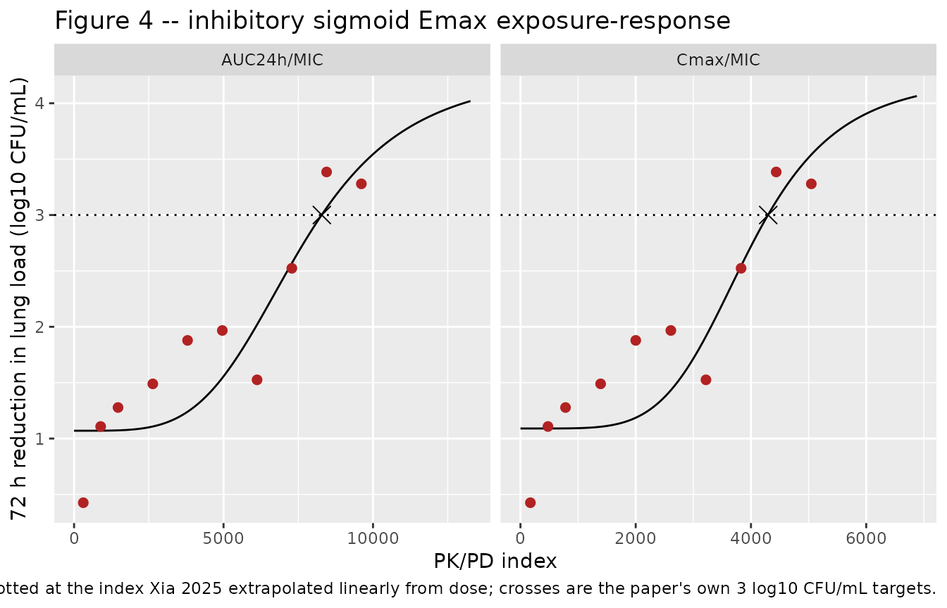
Replicate Figure 4: the exposure-response relationships
Figure 4 plots the 72 h reduction against AUC24h/MIC
(panel A, R^2 = 0.83) and Cmax/MIC (panel B, R^2 = 0.84).
Xia 2025 formed the index for the six doses it did not study
pharmacokinetically by linear extrapolation of the three measured dose
groups, giving AUC24h = 0.2271 * dose + 0.6015 (R^2 =
0.9978) and Cmax = 0.119 * dose + 0.3374 (R^2 =
0.9821).
Both parameterisations of Table 2 are reproduced below; only the AUC24h/MIC one is packaged, because a running Cmax is not an ODE quantity and because Xia 2025 designates AUC/MIC “as the most important parameter for evaluation”.
table2 <- tibble::tribble(
  ~index,        ~e0,   ~emax, ~ec50,    ~hill, ~r2,   ~target3log,
  "AUC24h/MIC",  1.07,  4.29,  7526.81,  4.22,  0.83,  8288.29,
  "Cmax/MIC",    1.09,  4.24,  3945.62,  5.09,  0.84,  4299.30
)

sigmoid <- function(ce, e0, emax, ec50, hill) {
  e0 + (emax - e0) * ce^hill / (ec50^hill + ce^hill)
}

mic_value <- 0.001953125
observed_index <- observed_pd |>
  transmute(
    dose,
    reduction,
    `AUC24h/MIC` = (0.2271 * dose + 0.6015) / mic_value,
    `Cmax/MIC` = (0.119 * dose + 0.3374) / mic_value
  ) |>
  tidyr::pivot_longer(c(`AUC24h/MIC`, `Cmax/MIC`), names_to = "index", values_to = "ce")

curve_grid <- bind_rows(lapply(seq_len(nrow(table2)), function(i) {
  r <- table2[i, ]
  ce <- seq(0, 1.6 * r$target3log, length.out = 400)
  tibble::tibble(index = r$index, ce = ce,
                 e = sigmoid(ce, r$e0, r$emax, r$ec50, r$hill))
}))

targets <- table2 |> transmute(index, ce = target3log, e = 3)

ggplot(curve_grid, aes(ce, e)) +
  geom_hline(yintercept = 3, linetype = "dotted") +
  geom_line() +
  geom_point(data = observed_index, aes(ce, reduction), colour = "firebrick", size = 2) +
  geom_point(data = targets, shape = 4, size = 4) +
  facet_wrap(~index, scales = "free_x") +
  labs(
    x = "PK/PD index", y = "72 h reduction in lung load (log10 CFU/mL)",
    title = "Figure 4 -- inhibitory sigmoid Emax exposure-response",
    caption = paste(
      "Replicates Figure 4 of Xia 2025. Red points are the observed group means",
      "(supplementary mmc4.xlsx) plotted at the index Xia 2025 extrapolated",
      "linearly from dose; crosses are the paper's own 3 log10 CFU/mL targets."
    )
  )
# The single strictest check on the parameterisation: at the paper's own
# reported 3 log10 CFU/mL target index, BOTH fits must return exactly 3.
at_target <- table2 |>
  mutate(e_at_target = sigmoid(target3log, e0, emax, ec50, hill))

at_target |>
  select(index, target3log, e_at_target, r2) |>
  mutate(e_at_target = round(e_at_target, 4)) |>
  dplyr::rename(
    "PK/PD index" = index,
    "Reported index at a 3 log10 drop" = target3log,
    "Model effect at that index" = e_at_target,
    "Reported R^2" = r2
  ) |>
knitr::kable(caption = "Xia 2025 Table 2: the 3 log10 CFU/mL target is an answer key for the parameterisation.")| PK/PD index | Reported index at a 3 log10 drop | Model effect at that index | Reported R^2 |
|---|---|---|---|
| AUC24h/MIC | 8288.29 | 3.0029 | 0.83 |
| Cmax/MIC | 4299.30 | 3.0037 | 0.84 |
stopifnot(max(abs(at_target$e_at_target - 3)) < 0.005)

# The packaged model's ini() must be the AUC24h/MIC row of Table 2.
stopifnot(
  abs(mod$theta[["e0"]] - 1.07) < 1e-9,
  abs(exp(mod$theta[["lemax"]]) - 4.29) < 1e-9,
  abs(exp(mod$theta[["lec50"]]) - 7526.81) < 1e-6,
  abs(exp(mod$theta[["lhill"]]) - 4.22) < 1e-9
)

# The zero-exposure asymptote is what Results quotes as the 0 mg/kg decrease.
stopifnot(all(abs(sigmoid(0, table2$e0, table2$emax, table2$ec50, table2$hill) -
                    c(1.07, 1.09)) < 1e-9))
Substituting Table 2 into the equation at the paper’s own reported
targets returns 3.003 and 3.004 log10 CFU/mL. That only holds if the
Table 2 row labelled Emax is the
zero-exposure effect and the row labelled
E0 is the maximum effect – the inversion
Xia 2025 states in Materials and methods and repeats in Results. No
other assignment of the two rows reproduces the targets.
Reproducing the recommended dose
Xia 2025’s formula (2), after setting fu = 1 and
F = 1 because total rather than free plasma concentrations
were measured, is
Dose = (AUC/MIC)breakpoint x MIC90 x Cl_per_hour / (fu x F)
with MIC90 replaced by the S6 strain MIC for want of
enough isolates.
clf_mean <- exp(mod$theta[["lcl"]])
dose_formula <- table2$target3log[table2$index == "AUC24h/MIC"] * mic_value * clf_mean

# Independently, invert the packaged ODE model: what dose drives a 3 log10
# reduction over the three-day course?
reduction_at <- function(d) {
  s <- solve_arm(d, n_doses = 3L, tmax = 72, times = c(0, 72))
  s$log10cfu[1] - s$log10cfu[nrow(s)]
}
dose_model <- stats::uniroot(function(d) reduction_at(d) - 3, interval = c(1, 200))$root

tibble::tibble(
  route = c("Xia 2025 formula (2), reproduced",
            "Packaged ODE model inverted to a 3 log10 CFU/mL drop",
            "Xia 2025 reported"),
  dose = c(dose_formula, dose_model, 62.64)
) |>
  mutate(dose = round(dose, 3)) |>
  dplyr::rename("Route" = route, "Dose (mg/kg once daily x 3 days)" = dose) |>
knitr::kable(caption = "Reproducing the recommended dose of Xia 2025.")| Route | Dose (mg/kg once daily x 3 days) |
|---|---|
| Xia 2025 formula (2), reproduced | 62.635 |
| Packaged ODE model inverted to a 3 log10 CFU/mL drop | 62.585 |
| Xia 2025 reported | 62.640 |
Both routes land on the paper’s recommended 62.64 mg/kg once daily
for three consecutive days. The agreement between the closed-form
formula and the inverted ODE model is the end-to-end check that the
packaged PK, the derived Q/F, the index definition and the
exposure-response are all wired together as Xia 2025 intended.
Assumptions and deviations
-
lqis derived, not published. Xia 2025 prints no intercompartmental clearance and nok12/k21.Q/F = 0.42210 L/h/kgis the unique value consistent with the four printed disposition quantities (Cl/F,V1/F,V2/F,T1/2kel) of the Table 1 mean column; the derivation, the round-trip and three independent confirmations thatT1/2kelis the terminal half-life are shown above. This is an algebraic consequence of published values, not a fitted or borrowed number, but it is nonetheless a value the reader will not find in the article. -
The Table 2 row labels are inverted relative to
convention. Xia 2025 defines “Emax = mycoplasma load change in
the positive control group during 72 h” and “E0 = maximum antimicrobial
effect reached after 72 h of treatment”, which is the opposite of the
usual reading. The packaged parameters are named for their role
(
e0= zero-exposure effect = the paper’sEmaxrow = 1.07;emax= maximum effect = the paper’sE0row = 4.29). The paper’s own 3 log10 CFU/mL target indices confirm the assignment numerically to three significant figures for both indices. -
e0is a fitted asymptote, not the observed control. The untreated control actually fell by 0.43 +/- 0.10 log10 CFU/mL over 72 h (Results, and supplementarymmc4.xlsx), whereas the fitted zero-exposure asymptote is 1.07. Xia 2025 reports both numbers without reconciling them; the packaged model reproduces the fitted asymptote, because that is the quantity the exposure-response model is built from. A simulated untreated control therefore declines faster than the observed one. -
The mean parameter column, not per-dose-group fits.
Xia 2025 fitted each dose group separately and reported a Mean +/- SEM
column. The mean column is packaged because it is the parameter set the
paper’s own dose calculation uses.
Cl/Frises with dose (3.35 -> 3.94 -> 4.31 L/h/kg), so the exposure is not quite dose proportional and the mean-parameter model over-predicts AUC24h at 80 mg/kg by about 11% and under-predicts at 5 mg/kg by about 13%. The per-dose-group sets and their derivedQ/Fvalues are recorded inpopulation$notesfor anyone wanting to reproduce one dose group exactly. -
“AUC24h” in Xia 2025 is
Dose / (Cl/F).Dose / (Cl/F)reproduces every reported AUC24h to nine decimal places, and formula (2) inverts exactly this relation, so the model forms the index that way. The true 0-24 h integral of the fitted model is 0.34% smaller (the extrapolated tail); both are carried in the model (auc24andauc_0_24) and compared above. -
podo(depot)supplies the dose to the index. The index is computed from the amount of the most recent depot dose, so it follows the actual dosing record rather than a duplicated parameter. Simulate an untreated control with an explicitamt = 0dose record; with no dose record at allpodo()isNAand the whole trajectory isNA. -
Xia 2025 extrapolated the index linearly from dose; the
model does not. For the six dose levels without PK data the
paper used
AUC24h = 0.2271 * dose + 0.6015, which has a non-zero intercept and so assigns a finite exposure to the 0 mg/kg group. The packaged model instead uses its ownDose / (Cl/F), which is zero at zero dose. The Figure 4 replication above plots the observed points on the paper’s extrapolated axis so the figure matches the article; the Figure 2 replication uses the model’s own index. The difference is up to about 14% on the index axis at the studied doses. -
The Cmax/MIC parameterisation is reproduced but not packaged
as a model file. Both Table 2 columns are validated above, but
only AUC24h/MIC is built into the ODE model: a running Cmax is not an
ODE quantity, and Xia 2025 states that AUC/MIC is the index it regards
as most important. The Cmax/MIC coefficients are recorded in
population$notes. - The reported 89.53% %T>MIC comes from linear interpolation. Xia 2025’s 5 mg/kg profile crosses the MIC inside the 12 h gap between its last two samples. Interpolating that gap linearly on the observed means reproduces the reported 89.53% exactly; interpolating it log-linearly, as a first-order decay requires, gives 78.7%, which is what the model returns. The number affects none of the packaged parameters – Xia 2025 used it only to argue that %T>MIC saturates and cannot discriminate, a conclusion the model supports either way.
-
A data-entry artefact in the 30 mg/kg group.
Supplementary
mmc4.xlsxreports seven lung counts for the 30 mg/kg group but computes its mean reduction over eight rows, the missing count contributing a spurious reduction of 6.130 (the 0 h mean minus zero). The published mean reduction of 1.878 log10 CFU/mL is therefore inflated; recomputed over the seven available counts it is 1.271. The paper’s own value is used above so the figure matches what Xia 2025 fitted, and the SEM shown for that group (0.633) is the paper’s inflated one. This affects one of ten points on the exposure-response and none of the packaged parameters. -
log10_cfu0is the efficacy cohort’s baseline. 6.130 log10 CFU/mL (mmc4.xlsx) is the 0 h count of the cohort the reductions are measured against. The 5.88 +/- 0.03 log10 CFU/mL quoted in Results belongs to the separate infection-model validation cohort (mmc2.xlsx). - No between-subject variability and no residual error. Blood was drawn once per chick and lungs counted once per chick, so no individual profiles exist and the paper reports no variance components – only bioanalytical recovery and precision for the assay and R^2 = 0.83 for the sigmoid. Both residual SDs are fixed at 0 and the model carries no eta parameters; it is for typical-value simulation.
-
Bioavailability is not identifiable. Only
intramuscular doses were given, so every disposition parameter carries
the paper’s
/FandFis implicitly 1. Xia 2025 setsF = 1in formula (2) for the same reason. -
Resistance selection is not modelled. Isolates
recovered from the 60, 70 and 80 mg/kg groups had MICs one two-fold
dilution higher (0.00390625 ug/mL,
mmc3.xlsx). The model uses the parent-strain MIC throughout, as the exposure-response fit did; changemicto explore the shifted isolates. -
Air-sac lesion scores are not modelled. Xia 2025
also reports lesion scores by dose (
mmc1.xlsx, Figure 3), but fits no model to them – they are compared by one-way ANOVA only – so there is nothing to package.