Talquetamab (Gong 2025)
Source:vignettes/articles/Gong_2025_talquetamab.Rmd
Gong_2025_talquetamab.RmdModel and source
- Citation: Gong J, Zhou J, Yuan D, Ma X, Vishwamitra D, Hilder B, Masterson TJ, Tolbert J, Renaud T, Heuck C, Kane C, Samtani MN, Girgis S, Haddish-Berhane N, Berdeja J, Krishnan A, Ouellet D. Recommended phase II doses of talquetamab in patients with relapsed/refractory multiple myeloma from MonumenTAL-1: clinical pharmacology results. Clin Pharmacol Ther. 2025;118(4):954-966. doi:10.1002/cpt.70004
- Description: Two-compartment population pharmacokinetic model for talquetamab, a GPRC5D x CD3 bispecific antibody, in patients with relapsed/refractory multiple myeloma (Gong 2025, MonumenTAL-1 phase I/II; 5354 serum concentrations from 492 patients dosed intravenously or subcutaneously). Subcutaneous absorption is sequential zero-order (duration D1) into a depot then first-order (Ka) into the central compartment. Total clearance is CL(t) = CL0 * (CLPCT + (1 - CLPCT) * exp(-KDES * t)): a time-independent share CL0 * CLPCT plus a time-dependent share that decays from the start of treatment with first-order rate KDES. Body weight acts on CL0 and the central volume; non-IgG myeloma and ISS stage II or III act on CL0. The paper’s exposure-response analyses for response, survival and adverse events are graphical or logistic-regression summaries without a reusable model, so only the population PK model is encoded.
- Article (open access): https://doi.org/10.1002/cpt.70004
Talquetamab is a GPRC5D x CD3 bispecific T-cell engager approved for relapsed/refractory multiple myeloma (RRMM) at two subcutaneous recommended phase II doses (RP2Ds): 0.4 mg/kg weekly (QW) and 0.8 mg/kg every other week (Q2W), each preceded by step-up doses. Gong 2025 reports the clinical pharmacology of the phase I/II MonumenTAL-1 study, including a population PK model whose structure and estimates are given in Supporting Information Figure S5 and Table S5.
The model has two compartments, a sequential zero-order (duration
D1) then first-order (Ka) subcutaneous
absorption, and a clearance that declines over time from its value at
treatment start, CL0:
CLPCT is the fraction of CL0 that remains
at steady state. Gong 2025 attributes the decline to falling tumour
burden or target level, disease severity or cancer cachexia, as reported
for nivolumab, teclistamab and daratumumab.
Population
The population PK dataset held 5354 measurable serum talquetamab concentrations from 492 patients, 100 dosed intravenously and 392 subcutaneously. Patients had a median age of 65 years (range 33-86) and a median weight of 74.8 kg (range 40.2-143); 42.7% were female and 86.2% White. Baseline ISS stage was I in 44.1%, II in 33.5% and III in 20.9%; 50.2% had IgG myeloma (Gong 2025 Table S4, overall column).
pop <- rxode2::rxode(readModelDb("Gong_2025_talquetamab"))$population
#> ℹ parameter labels from comments will be replaced by 'label()'
str(pop, max.level = 1)
#> List of 15
#>  $ species         : chr "human"
#>  $ n_subjects      : int 492
#>  $ n_studies       : int 1
#>  $ age_range       : chr "33-86 years"
#>  $ age_median      : chr "65 years"
#>  $ weight_range    : chr "40.2-143 kg"
#>  $ weight_median   : chr "74.8 kg"
#>  $ sex_female_pct  : num 42.7
#>  $ race_ethnicity  : Named num [1:5] 86.2 8.7 2.2 0.4 2.4
#>   ..- attr(*, "names")= chr [1:5] "White" "Black" "Asian" "NHPI" ...
#>  $ disease_state   : chr "Relapsed/refractory multiple myeloma (IMWG criteria). Phase I patients were intolerant of or had progressed on "| __truncated__
#>  $ dose_range      : chr "Intravenous 0.0015-0.18 mg/kg QW and 0.0005-0.00338 mg/kg Q2W; subcutaneous 0.005-0.8 mg/kg QW, 0.8 and 1.2 mg/"| __truncated__
#>  $ regions         : chr "Multicenter international (USA 152 patients in the Figure 4 subgroup analysis; other regions not tabulated)."
#>  $ renal_function  : chr "Renal function >= 90 mL/min in 31.5%, 60 to < 90 in 45.9%, 30 to < 60 in 22.2%, < 30 in 0.4%."
#>  $ hepatic_function: chr "Normal in 84.1%, impaired (mild, moderate or severe) in 15.4%, not reported in 0.4%."
#>  $ notes           : chr "Baseline demographics from Gong 2025 Table S4, overall column (n = 492): 100 patients dosed intravenously and 3"| __truncated__
Source trace
Every value comes from Gong 2025 Table S5 (“Parameter estimates for final population PK model”) and its footnotes; the structure is Figure S5.
| Equation / parameter | Value | Source location |
|---|---|---|
lcl (CL0) |
2.08 L/day | Table S5, RSE 6.58% |
cl_exp_famp (CLPCT - 1) |
0.512 - 1 | Table S5 CLPCT = 0.512, RSE 4.32% |
lcl_exp_kdes (KDES) |
0.0229 1/day | Table S5, RSE 7.21% |
lvc (V1) |
4.30 L | Table S5, RSE 2.54% |
lq (Q) |
1.01 L/day | Table S5, RSE 6.10% |
lvp (V2) |
5.78 L | Table S5, RSE 8.59% |
lka (Ka) |
0.138 1/day | Table S5, RSE 5.47% |
lfdepot (F) |
0.619 | Table S5, RSE 4.58% |
ld1 (D1) |
0.142 day | Table S5, RSE 19.6% |
e_wt_cl |
0.672 | Table S5 “BWT on CL0”, footnote a |
e_wt_vc |
0.670 | Table S5 “BWT on V1”, footnote b |
e_mm_nigg_cl |
-0.547 | Table S5 “IgG or non-IgG on CL0”; footnote a factor 0.453 |
e_iss_ii_iii_cl |
0.318 | Table S5 “ISS II or III on CL0”; footnote a factor 1.318 |
etalcl, etacl_exp_famp,
etalvc, etalcl_exp_kdes, etalq,
etalvp, etalka, etalfdepot,
etald1
|
log(1 + CV^2) with CV 51.7, 59.7, 22.3, 67.4, 39.4, 82.8, 65.9, 80.8, 145.3% | Table S5 IIV column |
propSd |
0.220 | Table S5 “Proportional error (CV%)” |
CL0 = 2.08 (BWT/74.8)^0.672 0.453^{non-IgG} 1.318^{ISS II/III} |
n/a | Table S5 footnote a |
CL = CL0 CLPCT + CL0 (1 - CLPCT) exp(-0.0229 t) |
n/a | Table S5 footnote a; Figure S5 |
V1 = 4.30 (BWT/74.8)^0.670 |
n/a | Table S5 footnote b |
| 2 compartments, SC input zero-order over D1 into depot then Ka; IV into central | n/a | Results; Figure S5 |
Virtual cohort
Observed data are not public. Three arms of 150 virtual patients each are given the schedules simulated in Gong 2025 Figure 3:
- QW RP2D: step-up doses 0.01 and 0.06 mg/kg, then 0.4 mg/kg weekly.
- Q2W RP2D (studied): step-up doses 0.01, 0.06 and 0.3 mg/kg, then 0.8 mg/kg every 2 weeks.
- Q2W RP2D (approved): step-up doses 0.01, 0.06 and 0.4 mg/kg, then 0.8 mg/kg every 2 weeks.
Gong 2025 Figure 4 places the Q2W step-up doses on days -6, -4 and -2
before the first full dose on day 0. The QW step-up days are not
printed; days -4 and -2 match where the QW curve starts in Figure 3a.
The model clock starts at the first step-up dose, because
KDES acts on time since the first dose.
# set.seed() fixes the covariate draws below; rxode2's own random-effect draws
# are not reproducible across builds, so the checks downstream target medians
# and typical values rather than cohort extremes.
set.seed(20250701)
n_per_arm <- 150L

arms <- tibble::tribble(
  ~arm,                  ~stepup,              ~full, ~tau,
  "0.4 mg/kg QW",        c(0.01, 0.06),        0.4,   7,
  "0.8 mg/kg Q2W",       c(0.01, 0.06, 0.3),   0.8,   14,
  "0.8 mg/kg Q2W (0.4 step-up)", c(0.01, 0.06, 0.4), 0.8, 14
)

n_weeks_full <- 10    # long enough for the Q2W cycle 3 day 1 interval (days 56-70)

make_doses <- function(stepup, full, tau) {
  t_full0 <- 2 * length(stepup)                 # step-ups 2 days apart
  full_times <- seq(t_full0, t_full0 + 7 * n_weeks_full - tau, by = tau)
  tibble(
    time = c(seq(0, by = 2, length.out = length(stepup)), full_times),
    mgkg = c(stepup, rep(full, length(full_times))),
    t_c1d1 = t_full0
  )
}

# Covariates: Table S4 overall column. WT median 74.8 kg (range 40.2-143);
# ISS I/II/III 217/165/103 of the 485 with a stage; non-IgG 245 of 492.
subj <- tibble(
  id = seq_len(3L * n_per_arm),
  arm = rep(arms$arm, each = n_per_arm),
  WT = pmin(pmax(rlnorm(3L * n_per_arm, log(74.8), 0.22), 40.2), 143),
  iss = sample(c("I", "II", "III"), 3L * n_per_arm, replace = TRUE,
               prob = c(217, 165, 103) / 485),
  MM_NIGG = rbinom(3L * n_per_arm, 1L, 245 / 492)
) |>
  mutate(ISS_II = as.integer(iss == "II"), ISS_III = as.integer(iss == "III"))

dose_rows <- subj |>
  inner_join(
    arms |> rowwise() |> reframe(arm, make_doses(stepup, full, tau)),
    by = "arm", relationship = "many-to-many"
  ) |>
  mutate(amt = mgkg * WT, evid = 1L, cmt = "depot", rate = -2)

t_c1d1 <- dose_rows |> distinct(arm, t_c1d1)

obs_times <- seq(0, 6 + 7 * n_weeks_full, by = 0.25)
obs_rows <- subj |>
  tidyr::crossing(time = obs_times) |>
  mutate(amt = NA_real_, evid = 0L, cmt = "central", rate = NA_real_)

events <- bind_rows(dose_rows, obs_rows) |>
  arrange(id, time, desc(evid)) |>
  select(id, time, amt, rate, evid, cmt, WT, ISS_II, ISS_III, MM_NIGG)
Simulation
mod <- readModelDb("Gong_2025_talquetamab")

sim <- rxode2::rxSolve(mod, events = events, keep = c("WT", "MM_NIGG", "ISS_II", "ISS_III")) |>
  as.data.frame() |>
  left_join(subj |> select(id, arm), by = "id") |>
  left_join(t_c1d1, by = "arm") |>
  mutate(time_c1d1 = time - t_c1d1)
#> ℹ parameter labels from comments will be replaced by 'label()'

stopifnot(nrow(sim) > 0, all(sim$Cc >= 0, na.rm = TRUE))
Concentration-time profiles (replicates Figure 3)
prof <- sim |>
  filter(time_c1d1 <= 56) |>
  group_by(arm, time_c1d1) |>
  summarise(
    Q05 = quantile(Cc, 0.05), Q50 = median(Cc), Q95 = quantile(Cc, 0.95),
    .groups = "drop"
  )

prof_a <- prof |> filter(arm != "0.8 mg/kg Q2W (0.4 step-up)") |> mutate(panel = "(a) RP2Ds")
prof_b <- prof |> filter(arm != "0.4 mg/kg QW") |> mutate(panel = "(b) Q2W step-up schedules")

bind_rows(prof_a, prof_b) |>
  filter(Q50 > 0.5) |>
  ggplot(aes(time_c1d1 / 7, Q50, colour = arm, fill = arm)) +
  geom_ribbon(aes(ymin = pmax(Q05, 0.5), ymax = Q95), alpha = 0.2, colour = NA) +
  geom_line(linewidth = 0.7) +
  geom_hline(yintercept = 353, linetype = "dashed") +
  facet_wrap(~panel, ncol = 1) +
  scale_y_log10(limits = c(0.5, 1e4)) +
  labs(
    x = "Time since cycle 1 day 1 dose (weeks)",
    y = "Talquetamab concentration (ng/mL)",
    colour = NULL, fill = NULL,
    caption = "Replicates Figure 3 of Gong 2025: median and 90% interval. Dashed line: maximum EC90, 353 ng/mL."
  ) +
  theme(legend.position = "bottom")
#> Warning: Removed 51 rows containing missing values or values outside the scale range
#> (`geom_ribbon()`).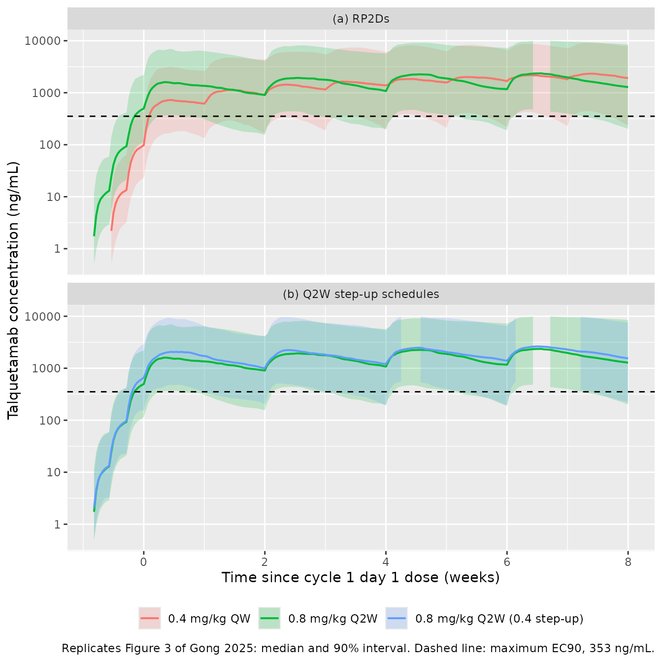
Both RP2D medians sit well above the maximum EC90 of 353 ng/mL after the first full dose, and the 5th percentile hovers around it, as Gong 2025 states. The two Q2W step-up schedules give overlapping profiles (Figure 3b).
ec90_tab <- sim |>
  filter(arm != "0.8 mg/kg Q2W (0.4 step-up)",
         time_c1d1 %in% c(7 * (1:8))) |>
  group_by(arm) |>
  summarise(
    `Median of predose concentrations, weeks 1-8 (ng/mL)` = median(Cc),
    `Predose samples above 353 ng/mL (%)` = 100 * mean(Cc >= 353),
    .groups = "drop"
  )
knitr::kable(ec90_tab, digits = 0)| arm | Median of predose concentrations, weeks 1-8 (ng/mL) | Predose samples above 353 ng/mL (%) |
|---|---|---|
| 0.4 mg/kg QW | 1313 | 88 |
| 0.8 mg/kg Q2W | 1363 | 89 |
PKNCA validation
Gong 2025 Table S3 reports phase I NCA at the RP2Ds after the cycle 1 day 1 and cycle 3 day 1 full doses: day 0 and day 42 for QW (21-day cycles) and day 0 and day 56 for Q2W (28-day cycles). Each dosing interval is passed to PKNCA as its own group with time re-zeroed at the dose.
windows <- tibble::tribble(
  ~arm,             ~interval,       ~start, ~tau,
  "0.4 mg/kg QW",   "Cycle 1 day 1", 0,      7,
  "0.4 mg/kg QW",   "Cycle 3 day 1", 42,     7,
  "0.8 mg/kg Q2W",  "Cycle 1 day 1", 0,      14,
  "0.8 mg/kg Q2W",  "Cycle 3 day 1", 56,     14
)

sim_nca <- windows |>
  rowwise() |>
  reframe(
    sim |>
      filter(arm == .env$arm, time_c1d1 >= start, time_c1d1 <= start + tau) |>
      mutate(interval = .env$interval, time_rel = time_c1d1 - .env$start)
  ) |>
  filter(!is.na(Cc)) |>
  mutate(treatment = paste(arm, interval, sep = ", ")) |>
  select(id, treatment, arm, interval, time_rel, Cc)

dose_nca <- sim_nca |>
  distinct(id, treatment, arm) |>
  left_join(subj |> select(id, WT), by = "id") |>
  mutate(time_rel = 0, amt = ifelse(arm == "0.4 mg/kg QW", 0.4, 0.8) * WT)

conc_obj <- PKNCA::PKNCAconc(as.data.frame(sim_nca), Cc ~ time_rel | treatment + id)
dose_obj <- PKNCA::PKNCAdose(as.data.frame(dose_nca), amt ~ time_rel | treatment + id)

intervals_all <- bind_rows(
  data.frame(treatment = c("0.4 mg/kg QW, Cycle 1 day 1", "0.4 mg/kg QW, Cycle 3 day 1"),
             start = 0, end = 7),
  data.frame(treatment = c("0.8 mg/kg Q2W, Cycle 1 day 1", "0.8 mg/kg Q2W, Cycle 3 day 1"),
             start = 0, end = 14)
) |>
  mutate(cmax = TRUE, tmax = TRUE, auclast = TRUE, cav = TRUE)

nca_res <- PKNCA::pk.nca(PKNCA::PKNCAdata(conc_obj, dose_obj, intervals = intervals_all))

# Table S3 trough = 'observed predose analyte concentration at the start of
# the dosing interval', i.e. the concentration at time_rel = 0.
predose <- sim_nca |> filter(time_rel == 0) |> select(treatment, id, ctrough = Cc)

nca_ind <- as.data.frame(nca_res) |>
  select(treatment, id, PPTESTCD, PPORRES) |>
  tidyr::pivot_wider(names_from = PPTESTCD, values_from = PPORRES) |>
  left_join(predose, by = c("treatment", "id")) |>
  mutate(auclast = auclast * 24)        # ng*day/mL -> ng*h/mL as in Table S3

stopifnot(nrow(nca_ind) == 4L * n_per_arm)
Side-by-side comparison with Table S3
Table S3 gives arithmetic means (and the median for tmax), so the simulated values are summarised the same way before the comparison.
published <- tibble::tribble(
  ~treatment,                     ~cmax, ~tmax, ~auclast, ~cav,  ~ctrough,
  "0.4 mg/kg QW, Cycle 1 day 1",  1568,  2.93,  178101,   1060,  178,
  "0.4 mg/kg QW, Cycle 3 day 1",  3799,  2.01,  607297,   3615,  2548,
  "0.8 mg/kg Q2W, Cycle 1 day 1", 2507,  2.83,  675764,   2011,  597,
  "0.8 mg/kg Q2W, Cycle 3 day 1", 4161,  2.85,  1021059,  3039,  1831
)

sim_summary <- nca_ind |>
  group_by(treatment) |>
  summarise(
    cmax = mean(cmax), tmax = median(tmax), auclast = mean(auclast),
    cav = mean(cav), ctrough = mean(ctrough), .groups = "drop"
  )

cmp <- nlmixr2lib::ncaComparisonTable(
  simulated = sim_summary,
  reference = published,
  by = "treatment",
  units = c(cmax = "ng/mL", tmax = "day", auclast = "ng*h/mL", cav = "ng/mL", ctrough = "ng/mL"),
  tolerance_pct = 20
)
knitr::kable(cmp, caption = "Simulated vs Gong 2025 Table S3 (means; tmax median). * differs by > 20%.")| NCA parameter | treatment | Reference | Simulated | % diff |
|---|---|---|---|---|
| Cmax (ng/mL) | 0.4 mg/kg QW, Cycle 1 day 1 | 1570 | 1080 | -31.4%* |
| Cmax (ng/mL) | 0.4 mg/kg QW, Cycle 3 day 1 | 3800 | 3130 | -17.7% |
| Cmax (ng/mL) | 0.8 mg/kg Q2W, Cycle 1 day 1 | 2510 | 2620 | +4.6% |
| Cmax (ng/mL) | 0.8 mg/kg Q2W, Cycle 3 day 1 | 4160 | 3970 | -4.5% |
| Tmax (day) | 0.4 mg/kg QW, Cycle 1 day 1 | 2.93 | 4 | +36.5%* |
| Tmax (day) | 0.4 mg/kg QW, Cycle 3 day 1 | 2.01 | 2.5 | +24.4%* |
| Tmax (day) | 0.8 mg/kg Q2W, Cycle 1 day 1 | 2.83 | 3.75 | +32.5%* |
| Tmax (day) | 0.8 mg/kg Q2W, Cycle 3 day 1 | 2.85 | 3.5 | +22.8%* |
| AUClast (ng*h/mL) | 0.4 mg/kg QW, Cycle 1 day 1 | 178000 | 145000 | -18.8% |
| AUClast (ng*h/mL) | 0.4 mg/kg QW, Cycle 3 day 1 | 607000 | 489000 | -19.4% |
| AUClast (ng*h/mL) | 0.8 mg/kg Q2W, Cycle 1 day 1 | 676000 | 640000 | -5.3% |
| AUClast (ng*h/mL) | 0.8 mg/kg Q2W, Cycle 3 day 1 | 1020000 | 1100000 | +7.6% |
| Cavg (ng/mL) | 0.4 mg/kg QW, Cycle 1 day 1 | 1060 | 861 | -18.8% |
| Cavg (ng/mL) | 0.4 mg/kg QW, Cycle 3 day 1 | 3620 | 2910 | -19.4% |
| Cavg (ng/mL) | 0.8 mg/kg Q2W, Cycle 1 day 1 | 2010 | 1900 | -5.3% |
| Cavg (ng/mL) | 0.8 mg/kg Q2W, Cycle 3 day 1 | 3040 | 3270 | +7.6% |
| Ctrough (ng/mL) | 0.4 mg/kg QW, Cycle 1 day 1 | 178 | 135 | -23.9%* |
| Ctrough (ng/mL) | 0.4 mg/kg QW, Cycle 3 day 1 | 2550 | 2480 | -2.6% |
| Ctrough (ng/mL) | 0.8 mg/kg Q2W, Cycle 1 day 1 | 597 | 720 | +20.6%* |
| Ctrough (ng/mL) | 0.8 mg/kg Q2W, Cycle 3 day 1 | 1830 | 2300 | +25.7%* |
The phase I NCA in Table S3 came from 13-33 patients per cell, with coefficients of variation of 40-90%, so differences of 20-40% from a population-model simulation of the whole phase I/II population are within the sampling noise of the observed means. The observed tmax comes from the sparse phase I schedule (samples on days 1, 2, 3, 4 and 8 or 9 after the dose; Table S1), so it is quantised differently from the 6-hour simulated grid and is expected to sit a day or so earlier. The 0.4 mg/kg QW cycle 1 values run lower than observed; they are also the most sensitive to the QW step-up timing, which Gong 2025 does not print (see Assumptions).
Terminal half-life (Results)
Gong 2025 reports a median terminal half-life of 7.56 days at
initial treatment and 12.2 days at steady
state. The individual terminal (beta-phase) half-life is
computed from each subject’s micro-constants with CL = CL0
at the start and CL = CL0 * CLPCT at steady state.
beta_half_life <- function(cl, vc, q, vp) {
  k10 <- cl / vc; k12 <- q / vc; k21 <- q / vp
  s <- k10 + k12 + k21
  beta <- (s - sqrt(s^2 - 4 * k10 * k21)) / 2
  log(2) / beta
}

hl <- sim |>
  group_by(id) |>
  slice(1) |>
  ungroup() |>
  mutate(
    clpct_i = 1 + cl_exp_famp_i,
    thalf_start = beta_half_life(cl0, vc, q, vp),
    thalf_ss = beta_half_life(cl0 * clpct_i, vc, q, vp)
  )

hl_tab <- tibble(
  Quantity = c("Median terminal half-life at initial treatment (day)",
               "Median terminal half-life at steady state (day)"),
  Simulated = c(median(hl$thalf_start), median(hl$thalf_ss)),
  Published = c(7.56, 12.2)
) |>
  mutate(`Difference (%)` = 100 * (Simulated - Published) / Published)
knitr::kable(hl_tab, digits = 2)| Quantity | Simulated | Published | Difference (%) |
|---|---|---|---|
| Median terminal half-life at initial treatment (day) | 8.01 | 7.56 | 6.00 |
| Median terminal half-life at steady state (day) | 12.38 | 12.20 | 1.46 |
Covariate effects on exposure (Figure 4)
Figure 4 of Gong 2025 reports the geometric-mean ratio of
Cavg,4weeks (the average concentration over the first 4
weeks of full doses) at the 0.8 mg/kg Q2W RP2D: 2.0 for
non-IgG vs IgG myeloma, 0.77 for ISS stage II and
0.71 for stage III vs stage I. Those are ratios of post
hoc exposures and carry the cohort’s covariate correlations; the
typical-value ratios below isolate each model effect.
typ_events <- function(nigg, iss23) {
  d <- make_doses(c(0.01, 0.06, 0.3), 0.8, 14)
  bind_rows(
    tibble(id = 1L, time = d$time, amt = d$mgkg * 74.8, rate = -2, evid = 1L, cmt = "depot"),
    tibble(id = 1L, time = seq(0, 6 + 28, by = 0.05), amt = NA_real_, rate = NA_real_,
           evid = 0L, cmt = "central")
  ) |>
    arrange(time, desc(evid)) |>
    mutate(WT = 74.8, MM_NIGG = nigg, ISS_II = iss23, ISS_III = 0L)
}

cavg4 <- function(nigg, iss23) {
  s <- rxode2::rxSolve(rxode2::zeroRe(mod), events = typ_events(nigg, iss23)) |>
    as.data.frame() |>
    filter(time >= 6, time <= 34)
  sum(diff(s$time) * (head(s$Cc, -1) + tail(s$Cc, -1)) / 2) / 28
}

ref <- cavg4(0L, 0L)
#> ℹ parameter labels from comments will be replaced by 'label()'
#> ℹ omega/sigma items treated as zero: 'etalcl', 'etacl_exp_famp', 'etalvc', 'etalcl_exp_kdes', 'etalq', 'etalvp', 'etalka', 'etalfdepot', 'etald1'
cov_tab <- tibble(
  Comparison = c("Non-IgG vs IgG myeloma", "ISS II or III vs ISS I"),
  `Typical-value ratio` = c(cavg4(1L, 0L) / ref, cavg4(0L, 1L) / ref),
  `Figure 4 GMR` = c("2.0 (1.8-2.1)", "0.77 (II); 0.71 (III)")
)
#> ℹ parameter labels from comments will be replaced by 'label()'
#> ℹ omega/sigma items treated as zero: 'etalcl', 'etacl_exp_famp', 'etalvc', 'etalcl_exp_kdes', 'etalq', 'etalvp', 'etalka', 'etalfdepot', 'etald1'
#> ℹ parameter labels from comments will be replaced by 'label()'
#> ℹ omega/sigma items treated as zero: 'etalcl', 'etacl_exp_famp', 'etalvc', 'etalcl_exp_kdes', 'etalq', 'etalvp', 'etalka', 'etalfdepot', 'etald1'
knitr::kable(cov_tab, digits = 2)| Comparison | Typical-value ratio | Figure 4 GMR |
|---|---|---|
| Non-IgG vs IgG myeloma | 1.79 | 2.0 (1.8-2.1) |
| ISS II or III vs ISS I | 0.79 | 0.77 (II); 0.71 (III) |
The non-IgG factor of 0.453 on CL0 gives a typical-value
ratio at the lower end of the published interval, and the single pooled
ISS factor of 1.318 lands between the stage II and stage III ratios, as
expected when one coefficient serves both stages.
The typical-value Cavg,4weeks at the Q2W RP2D for a 74.8
kg IgG, ISS I patient is 1468 ng/mL. Gong 2025 Figure 5a shows the RP2D
exposures spanning roughly 100 to 5000 ng/mL with medians near 1000-1500
ng/mL.
sim |>
  filter(arm != "0.8 mg/kg Q2W (0.4 step-up)", time_c1d1 >= 0, time_c1d1 <= 28) |>
  group_by(arm, id) |>
  summarise(cavg4 = sum(diff(time_c1d1) * (head(Cc, -1) + tail(Cc, -1)) / 2) / 28,
            .groups = "drop") |>
  group_by(arm) |>
  summarise(median = median(cavg4), Q25 = quantile(cavg4, 0.25),
            Q75 = quantile(cavg4, 0.75), .groups = "drop") |>
knitr::kable(digits = 0, caption = "Simulated Cavg,4weeks (ng/mL); compare the Figure 5a box plots.")| arm | median | Q25 | Q75 |
|---|---|---|---|
| 0.4 mg/kg QW | 1107 | 614 | 2141 |
| 0.8 mg/kg Q2W | 1454 | 782 | 2867 |
Steady state (Results)
Gong 2025 reports that steady state (90% of the steady-state
concentration) was reached at week 16 for both RP2Ds. Because the
clearance falls with KDES (half-time 30 days), steady state
depends on both accumulation and the clearance decline. The
typical-value interval average for an IgG, ISS I patient is compared
with its value after one year.
ss_profile <- function(stepup, full, tau) {
  d <- make_doses(stepup, full, tau)
  t0 <- d$t_c1d1[1]
  full_times <- seq(t0, t0 + 400, by = tau)
  ev <- bind_rows(
    tibble(time = c(seq(0, by = 2, length.out = length(stepup)), full_times),
           amt = c(stepup, rep(full, length(full_times))) * 74.8,
           rate = -2, evid = 1L, cmt = "depot"),
    tibble(time = seq(0, t0 + 400, by = 0.25), amt = NA_real_, rate = NA_real_,
           evid = 0L, cmt = "central")
  ) |>
    arrange(time, desc(evid)) |>
    mutate(id = 1L, WT = 74.8, MM_NIGG = 0L, ISS_II = 0L, ISS_III = 0L)
  s <- rxode2::rxSolve(rxode2::zeroRe(mod), events = ev) |> as.data.frame()
  tibble(start = head(full_times, -1)) |>
    rowwise() |>
    mutate(cavg = {
      w <- s[s$time >= start & s$time <= start + tau, ]
      sum(diff(w$time) * (head(w$Cc, -1) + tail(w$Cc, -1)) / 2) / tau
    }) |>
    ungroup() |>
    mutate(week = (start - t0) / 7)
}

ss <- bind_rows(
  ss_profile(c(0.01, 0.06), 0.4, 7) |> mutate(arm = "0.4 mg/kg QW"),
  ss_profile(c(0.01, 0.06, 0.3), 0.8, 14) |> mutate(arm = "0.8 mg/kg Q2W")
) |>
  group_by(arm) |>
  mutate(frac_ss = cavg / cavg[week == max(week[week <= 52])]) |>
  ungroup()
#> ℹ parameter labels from comments will be replaced by 'label()'
#> ℹ omega/sigma items treated as zero: 'etalcl', 'etacl_exp_famp', 'etalvc', 'etalcl_exp_kdes', 'etalq', 'etalvp', 'etalka', 'etalfdepot', 'etald1'
#> ℹ parameter labels from comments will be replaced by 'label()'
#> ℹ omega/sigma items treated as zero: 'etalcl', 'etacl_exp_famp', 'etalvc', 'etalcl_exp_kdes', 'etalq', 'etalvp', 'etalka', 'etalfdepot', 'etald1'

ss_week <- ss |>
  filter(frac_ss >= 0.9) |>
  group_by(arm) |>
  summarise(`First week with Cavg >= 90% of the 1-year value` = min(week), .groups = "drop")
knitr::kable(ss_week)| arm | First week with Cavg >= 90% of the 1-year value |
|---|---|
| 0.4 mg/kg QW | 14 |
| 0.8 mg/kg Q2W | 14 |
ggplot(ss |> filter(week <= 40), aes(week, frac_ss, colour = arm)) +
  geom_step() +
  geom_hline(yintercept = 0.9, linetype = "dashed") +
  geom_vline(xintercept = 16, linetype = "dotted") +
  labs(x = "Week of full-dose treatment", y = "Interval Cavg / 1-year value",
       colour = NULL, caption = "Dotted line: week 16, where Gong 2025 reports steady state.")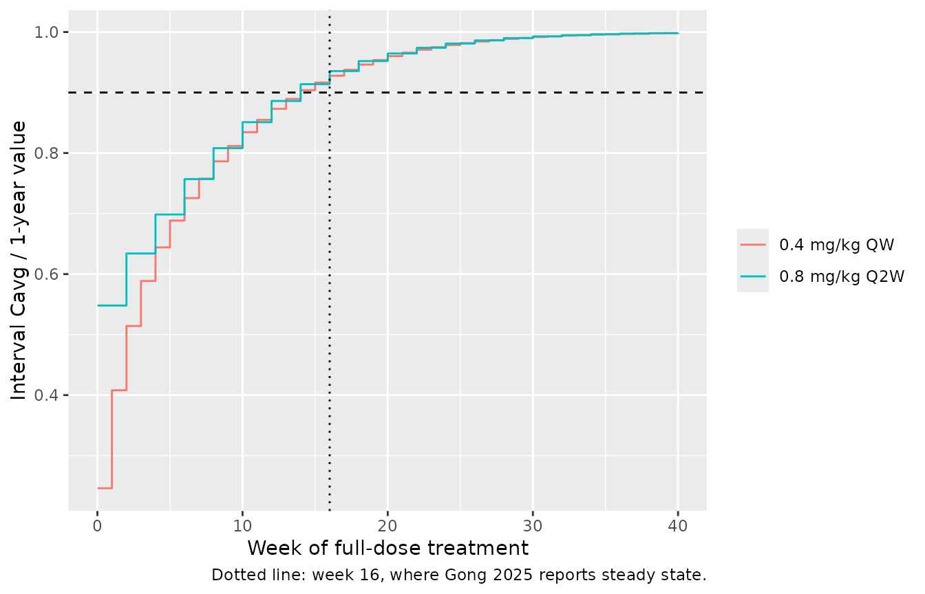
The typical patient reaches 90% of the steady-state interval average
a little before week 16; Gong 2025’s figure is a population summary
across patients whose KDES varies with a 67% CV, so a later
population-level time is expected.
Validation gate
stopifnot(
  # Half-lives: a mis-transcribed CL0, CLPCT, Q or V2 moves these by tens of percent.
  abs(hl_tab$`Difference (%)`[1]) < 20,
  abs(hl_tab$`Difference (%)`[2]) < 20,
  # Covariate effects (typical value, deterministic).
  abs(cov_tab$`Typical-value ratio`[1] / 2.0 - 1) < 0.15,
  cov_tab$`Typical-value ratio`[2] > 0.68, cov_tab$`Typical-value ratio`[2] < 0.80,
  # Exposure centre: simulated mean Cavg in every Table S3 cell within a factor
  # of 1.6 of the published mean.
  all(abs(log(sim_summary$cav / published$cav[match(sim_summary$treatment, published$treatment)])) < log(1.6))
)
Assumptions and deviations
- IIV distribution of the fractional parameters. Gong 2025 Methods state that every random effect was log-normal, and Table S5 reports IIV as CV% on CLPCT (59.7%) and F (80.8%) as on the other parameters. They are encoded log-normally as stated, so some simulated patients have F > 1 or CLPCT > 1 (a clearance that rises rather than falls over time). A logit transform, common for fractions, is not described and was not substituted.
-
CV to variance. The paper does not state its CV
definition; the exact log-normal relation
omega^2 = log(1 + CV^2)is used for every eta. No covariances are reported, so the etas are independent. -
CLPCT parameterisation. The model stores CLPCT as
the registered signed amplitude
cl_exp_famp = CLPCT - 1, socl = CL0 * (1 + cl_exp_famp * (1 - exp(-KDES t))); this is algebraically identical to Table S5 footnote a. The CLPCT eta multiplies CLPCT itself. -
Pooled ISS effect. Gong 2025 estimates one factor
(1.318) for ISS stage II or III; the model applies it as
(1 + 0.318 * (ISS_II + ISS_III)). Figure 4’s separate 0.77 and 0.71 ratios come from post hoc exposures, not from separate model terms. -
Residual error. Table S5 lists “Proportional error
(CV%)” as 0.220; it is read as a 22% proportional error
(
propSd = 0.220). - Step-up timing. The QW step-up days (-4 and -2 before the first full dose) are read from where the QW curve starts in Figure 3a; the Q2W days (-6, -4, -2) are printed in the Figure 4 caption.
- Dose level. Phase I used 0.405 mg/kg QW and phase II 0.4 mg/kg; 0.4 mg/kg is simulated throughout, a 1.2% difference.
- Exposure-response models. The ORR logistic/Emax regressions, the Kaplan-Meier analyses and the safety quartile analyses are not encoded: their coefficients are not reported (Table S6 gives only odds ratios for MM subtype and extramedullary plasmacytoma, with a flat exposure term).