Fractal kinetics in population PK (Jung 2023)
Source:vignettes/articles/Jung_2023_fractal_kinetics.Rmd
Jung_2023_fractal_kinetics.Rmd
library(nlmixr2lib)
library(rxode2)
#> rxode2 5.1.8 using 2 threads (see ?getRxThreads)
#>   no cache: create with `rxCreateCache()`
library(dplyr)
#>
#> Attaching package: 'dplyr'
#> The following objects are masked from 'package:stats':
#>
#>     filter, lag
#> The following objects are masked from 'package:base':
#>
#>     intersect, setdiff, setequal, union
library(tidyr)
library(ggplot2)
library(PKNCA)
#>
#> Attaching package: 'PKNCA'
#> The following object is masked from 'package:stats':
#>
#>     filter
Fractal kinetics applied to five population PK models
Jung 2023 (Pharmaceutics 15(1):304, doi:10.3390/pharmaceutics15010304) is a methods paper with a concrete deliverable: it takes five previously fitted population PK models, replaces one first-order rate constant in each with a fractal (Kopelman) rate, re-estimates every model, and reports the full converged parameter set for all five. This vignette implements the five re-estimated (fractal) models and checks them.
The fractal modification replaces a constant first-order rate constant by a time-dependent instantaneous rate coefficient (Jung 2023 Equation 1):
where q carries the units of a first-order rate constant
and h is a unitless heterogeneity exponent
bounded in [0, 1]. Setting h = 0 recovers
ordinary constant-rate (Fick) kinetics; increasing h
front-loads the process, producing a burst followed by a long tail. The
physical motivation is a reaction on a fractal or otherwise
non-homogeneous support, where the effective rate falls as the readily
accessible material is consumed.
In every one of the five cases the fractal rate is applied to an absorption or release step, never to disposition.
mCase1 <- readModelDb("Jung_2023_donepezil_singledose")
mCase2 <- readModelDb("Jung_2023_donepezil_multipledose")
mCase3 <- readModelDb("Jung_2023_im_depot")
mCase4 <- readModelDb("Jung_2023_HL2351")
mCase5 <- readModelDb("Jung_2023_anakinra")
The five cases
| Case | Model | Drug | Structure | Fractal rate on |
|---|---|---|---|---|
| 1 | Jung_2023_donepezil_singledose | donepezil | 2-cmt, oral + patch, 2 transit | patch reservoir release |
| 2 | Jung_2023_donepezil_multipledose | donepezil (inferred) | 2-cmt, oral + patch, 1 transit | patch reservoir release (reset per dose) |
| 3 | Jung_2023_im_depot | not disclosed | 2-cmt IM, fast + slow (Savic transit) | fast IM release |
| 4 | Jung_2023_HL2351 | HL2351 | 2-cmt QSS-TMDD + FcRn recycling | absorption site to plasma |
| 5 | Jung_2023_anakinra | anakinra | 1-cmt QSS-TMDD | absorption from injection site |
Jung 2023 Table 2 reports the fit statistics. The fractal parameter
improved the objective function in every case, but by the corrected AIC
it was worth the extra parameter in only four of the five: Case 3’s
h estimated to 0.0268, an exponent so close to zero that
the model reduces to its own base model.
| Case | Subjects | Observations | OFV base | OFV fractal | d OFV | d AICc |
|---|---|---|---|---|---|---|
| 1 | 18 | 383 | 1443.70 | 1410.08 | -33.62 | -31.47 |
| 2 | 44 | 3024 | 13977.10 | 13592.00 | -385.10 | -381.06 |
| 3 | 20 | 339 | 2155.43 | 2153.54 | -1.89 | 2.55 |
| 4 | 40 | 472 | 1556.43 | 1539.64 | -16.79 | -14.58 |
| 5 | 8 | 93 | 358.47 | 350.13 | -8.34 | -3.12 |
What the fractal exponent does
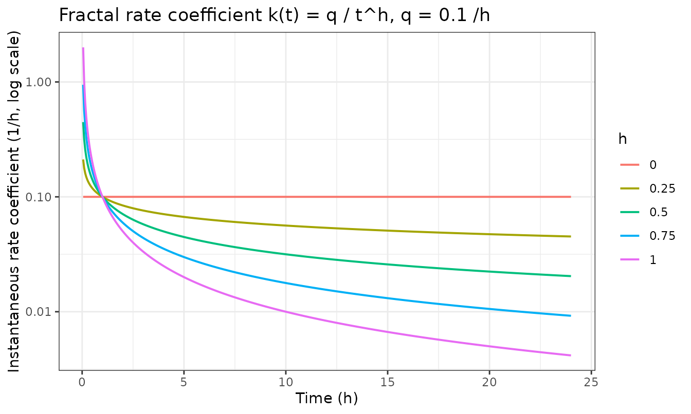
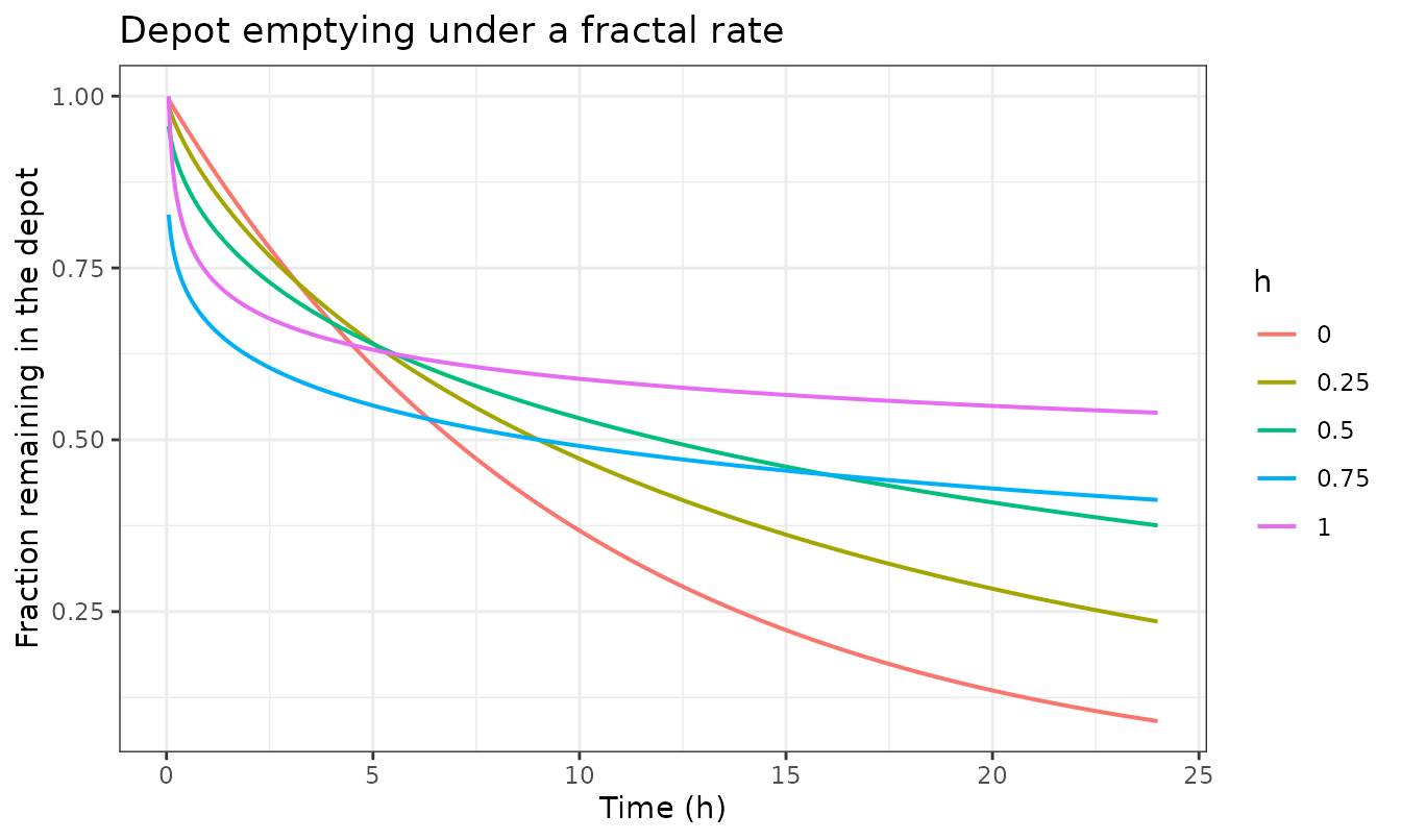
This reproduces the mechanism illustrated in Jung 2023 Figures 2 and
3: the instantaneous rate coefficient for a range of h, and
the amount-remaining profile it produces from a single depot.
h = 0 is a straight exponential decay; larger
h gives an increasingly sharp initial loss followed by a
markedly slower tail.
Source trace
Jung 2023’s main text contains no parameter values –
Table 2 carries only OFV, AIC and AICc. Every estimate in the five model
files comes from the Supplementary Materials, which contain Tables S1-S5
(one estimate table per case) and Codes S1-S11 (the NONMEM control
streams, base and fractal for each case). Where the two disagree the
control stream is authoritative, because its $THETA block
carries the converged values to six significant figures while the tables
are rounded to three; the two agree everywhere except the single Case 3
residual-error discrepancy noted under Errata.
| Case | Quantity | Source |
|---|---|---|
| 1 | Structural, IIV, residual error | Table S1 (rounded), Code S3 $THETA / $OMEGA (converged) |
| 1 | ODE structure, fractal rate site | Code S3 $MODEL / $DES / $PK; Figure S1 |
| 2 | Structural, IIV, residual error | Table S2 (rounded), Code S5 $THETA / $OMEGA (converged) |
| 2 | ODE structure, per-dose reset, tau | Code S5 $MODEL / $DES / $PK; Figure S2 |
| 3 | Structural, IIV, residual error | Table S3 (rounded), Code S7 $THETA / $OMEGA (converged) |
| 3 | ODE structure, Savic transit chain | Code S7 $MODEL / $DES / $PK; Figure S3 |
| 4 | Structural, IIV, residual error | Table S4 (rounded), Code S9 $THETA / $OMEGA (converged) |
| 4 | ODE structure, QSS-TMDD + FcRn | Code S9 $MODEL / $DES / $PK / $ERROR; Figure S4 |
| 5 | Structural, IIV, residual error | Table S5 (rounded), Code S11 $THETA / $OMEGA (converged) |
| 5 | ODE structure, QSS-TMDD | Code S11 $MODEL / $DES / $PK / $ERROR; Figure S5 |
| NA | Subject and observation counts | Jung 2023 main text Table 2 |
| NA | Fit statistics (OFV / AIC / AICc) | Jung 2023 main text Table 2 |
| NA | Case 1 study design and demographics | Jung 2022, doi:10.3390/pharmaceutics14020244 (ref [3]) |
| NA | Case 4 / 5 study design and demographics | Ngo 2020, doi:10.1002/psp4.12555 (ref [16]) |
Every ini() entry in the five model files additionally
carries an in-file comment naming its $THETA /
$OMEGA index and the matching table row, so the provenance
of individual numbers is auditable at the line level.
Verification
The checks below are deliberately built from values printed in the paper (clearances from Tables S1-S5, the transit mean time, the QSS constants), never from variables read back out of the model object. A gate assembled from the model’s own parameters cannot fail even when the model is wrong.
Jung 2023 reports no non-compartmental summary statistics – no Cmax,
Tmax, AUC or half-life tables – so there is nothing to compare a
simulated NCA against. The NCA below therefore serves a different
purpose: for the three linear cases it tests the dose-exposure identity
AUC(0-inf) = Dose / CL against the printed
clearance, which is a genuine end-to-end check of the ODE wiring, the
bioavailability routing and the concentration unit scaling all at
once.
Cases 1 and 2: donepezil, oral and transdermal
Typical-value profiles (inter-individual variability suppressed with
rxode2::zeroRe()) for the single-dose model.
ev1_oral <- rxode2::et(amt = 10, cmt = "depot_oral", time = 0) |>
  rxode2::et(seq(0, 312, by = 1), cmt = "central")
ev1_patch <- rxode2::et(amt = 108, cmt = "depot_td", time = 0) |>
  rxode2::et(seq(0, 312, by = 1), cmt = "central")

s1_oral  <- rxode2::rxSolve(rxode2::zeroRe(mCase1), ev1_oral,  returnType = "data.frame")
#> ℹ parameter labels from comments will be replaced by 'label()'
#> ℹ omega/sigma items treated as zero: 'etalka', 'etalcl', 'etalvc', 'etalktr'
s1_patch <- rxode2::rxSolve(rxode2::zeroRe(mCase1), ev1_patch, returnType = "data.frame")
#> ℹ parameter labels from comments will be replaced by 'label()'
#> ℹ omega/sigma items treated as zero: 'etalka', 'etalcl', 'etalvc', 'etalktr'

case1 <- bind_rows(
  mutate(s1_oral,  arm = "Oral 10 mg"),
  mutate(s1_patch, arm = "Patch 108 mg")
)

ggplot(case1, aes(time, Cc, colour = arm)) +
  geom_line(linewidth = 0.7) +
  labs(x = "Time (h)", y = "Donepezil (ng/mL)", colour = NULL,
       title = "Case 1: single-dose donepezil, typical-value profiles") +
  theme_bw()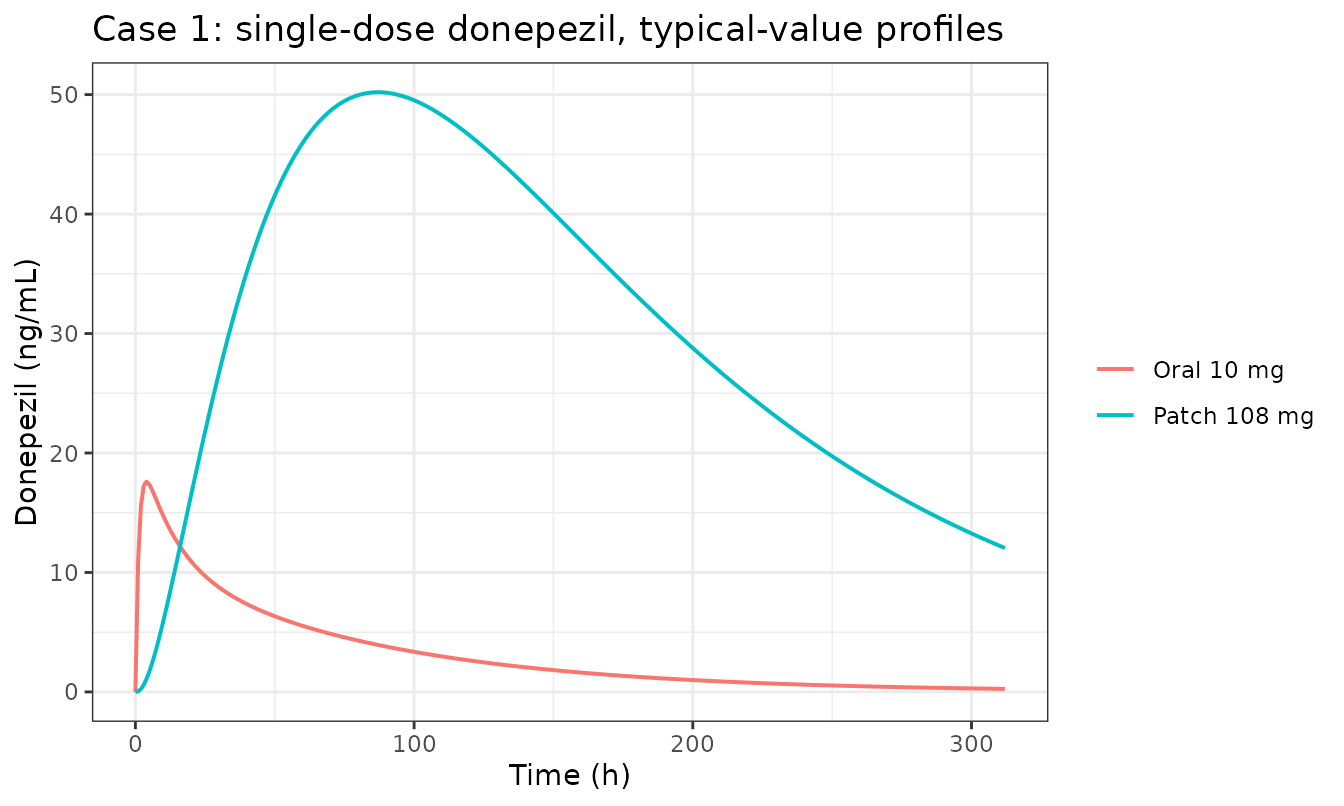
The oral arm is a plain first-order absorption into a linear
two-compartment disposition, so its total exposure must satisfy
AUC = Dose / CL using the clearance printed in Table S1
(9.68 L/h). Dose is 10 mg and concentrations are ng/mL, so the expected
AUC is
10 mg / 9.68 L/h = 1.0331 mg*h/L = 1033.1 ng*h/mL.
# Trapezoidal AUC to 312 h plus the terminal tail, from the typical-value solve.
auc_with_tail <- function(d) {
  a_obs <- sum(diff(d$time) * (head(d$Cc, -1) + tail(d$Cc, -1)) / 2)
  # terminal slope from the last quarter of the profile
  tailrows <- tail(d, max(10L, floor(nrow(d) / 4)))
  lz <- -stats::coef(stats::lm(log(Cc) ~ time, data = tailrows))[["time"]]
  a_obs + tail(d$Cc, 1) / lz
}

cl_printed_case1 <- 9.68           # Jung 2023 Table S1, fractal column, CL (L/h)
auc_expected1    <- 10 / cl_printed_case1 * 1000   # mg / (L/h) -> ng*h/mL
auc_observed1    <- auc_with_tail(s1_oral)

c(expected = auc_expected1, observed = auc_observed1,
  pct_diff = 100 * (auc_observed1 - auc_expected1) / auc_expected1)
#>     expected     observed     pct_diff
#> 1033.0578512 1031.5861549   -0.1424602

stopifnot(abs(auc_observed1 - auc_expected1) / auc_expected1 < 0.02)
Case 2 is the multiple-dose model, and the only one of the five whose fractal clock restarts at every dose. The control stream (Code S5) tracks the time of the most recent dosing record and forms the release coefficient from the elapsed time since it, so each new patch begins its release profile afresh rather than continuing to decay on an absolute clock. The check below is the structural one: the fraction of the reservoir released in the first 24 h must be the same for every patch.
ev2 <- rxode2::et(amt = 10, cmt = "depot_oral", time = 0, ii = 24, addl = 6) |>
  rxode2::et(amt = 108, cmt = "depot_td", time = 168) |>
  rxode2::et(amt = 108, cmt = "depot_td", time = 888) |>
  rxode2::et(amt = 108, cmt = "depot_td", time = 1608) |>
  rxode2::et(seq(0, 2496, by = 2), cmt = "central")

s2 <- rxode2::rxSolve(rxode2::zeroRe(mCase2), ev2, returnType = "data.frame")
#> ℹ parameter labels from comments will be replaced by 'label()'
#> ℹ omega/sigma items treated as zero: 'etalka', 'etalcl', 'etalvc', 'etalq', 'etalktr', 'etah_abs'

released_24h <- vapply(c(168, 888, 1608), function(td) {
  w <- s2[s2$time >= td & s2$time <= td + 24, ]
  1 - tail(w$depot_td, 1) / w$depot_td[1]
}, numeric(1))

released_24h
#> [1] 0.9898086 0.9898086 0.9898086

# Every patch must release the same fraction in its first 24 h. If the clock ran
# on absolute time instead of time-after-dose, the later patches would release
# dramatically less and this spread would be large.
stopifnot(diff(range(released_24h)) < 1e-6)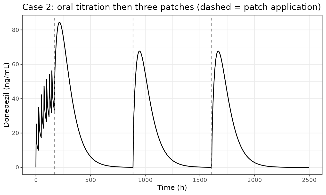
Case 3: controlled-release intramuscular depot
Case 3 splits the dose between a fast-release depot given the fractal
rate and a slow-release arm routed through a Savic transit chain. The
transit chain is the part with a hard, printed target: the chain’s
input rate into the slow depot is a gamma density in
elapsed time whose mode is the mean transit time, so it must peak at
t = MTT. Table S3 prints MTT = 136 h.
The quantity to test is the input rate inpt, not the
depot2 state. depot2 accumulates that input
while simultaneously draining at ka_slow, so its own
maximum falls well after MTT (about 173 h here) and would
not test the transit chain at all.
ev3 <- rxode2::et(amt = 1000, cmt = "depot", time = 0) |>
  rxode2::et(seq(0, 672, by = 1), cmt = "central")
s3 <- rxode2::rxSolve(rxode2::zeroRe(mCase3), ev3, returnType = "data.frame")
#> ℹ parameter labels from comments will be replaced by 'label()'
#> ℹ omega/sigma items treated as zero: 'etalvc', 'etalq', 'etalka_fast', 'etalntr', 'etalfrac', 'etah_abs'

mtt_printed  <- 136           # Jung 2023 Table S3, fractal column, MTT (h)
t_peak_input <- s3$time[which.max(s3$inpt)]

c(mtt_printed = mtt_printed, simulated_input_peak_h = t_peak_input)
#>            mtt_printed simulated_input_peak_h
#>                    136                    135

# The transit input rate must peak at t = MTT. The observation grid is 1 h, so
# allow the grid resolution plus one step.
stopifnot(abs(t_peak_input - mtt_printed) <= 2)
The transit chain also has a conservation property: integrated over
all time the input must deliver exactly the slow-arm fraction of the
dose, (1 - FRAC) * Dose, with FRAC = 0.172
printed in Table S3.
frac_printed <- 0.172         # Jung 2023 Table S3, fractal column, FRAC
dose3 <- 1000
delivered <- sum(diff(s3$time) * (head(s3$inpt, -1) + tail(s3$inpt, -1)) / 2)
expected3 <- (1 - frac_printed) * dose3

c(expected = expected3, delivered = delivered,
  pct_diff = 100 * (delivered - expected3) / expected3)
#>     expected    delivered     pct_diff
#> 828.00000000 828.61436718   0.07419893

stopifnot(abs(delivered - expected3) / expected3 < 0.01)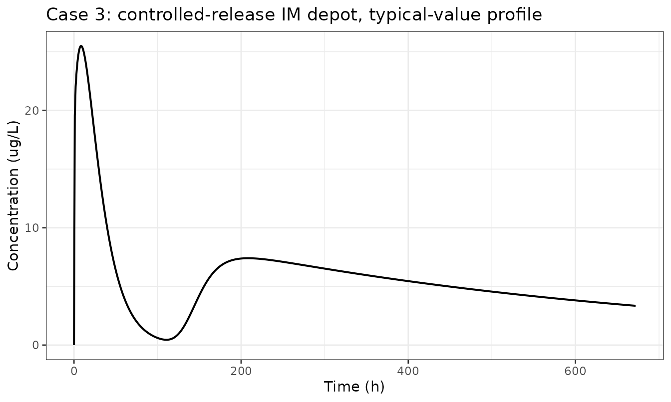
Cases 4 and 5: target-mediated disposition
Both TMDD cases carry the drug as a total amount and recover the free concentration through a quasi-steady-state quadratic. Two properties must hold identically, whatever the parameter values: free concentration never exceeds total, and as the total rises far above the target capacity the free fraction approaches one. These are structural checks on the QSS algebra rather than on any single estimate.
NMOL_PER_MG_HL2351 <- 1e6 / 97000   # MW ~97 kDa -> 1 mg = 10.31 nmol
wt <- 70

case4 <- lapply(c(1, 4, 12), function(mgkg) {
  ev <- rxode2::et(amt = mgkg * wt * NMOL_PER_MG_HL2351, cmt = "depot", time = 0) |>
    rxode2::et(seq(0, 672, by = 2), cmt = "central")
  rxode2::rxSolve(rxode2::zeroRe(mCase4), ev, returnType = "data.frame") |>
    mutate(dose = paste0(mgkg, " mg/kg"))
}) |> bind_rows()
#> ℹ parameter labels from comments will be replaced by 'label()'
#> ℹ omega/sigma items treated as zero: 'etalka1', 'etalka2', 'etalkrec', 'etalkdeg', 'etalkup', 'etaltlag', 'etalcl'
#> ℹ parameter labels from comments will be replaced by 'label()'
#> ℹ omega/sigma items treated as zero: 'etalka1', 'etalka2', 'etalkrec', 'etalkdeg', 'etalkup', 'etaltlag', 'etalcl'
#> ℹ parameter labels from comments will be replaced by 'label()'
#> ℹ omega/sigma items treated as zero: 'etalka1', 'etalka2', 'etalkrec', 'etalkdeg', 'etalkup', 'etaltlag', 'etalcl'

# Cc is the FREE concentration; central/vc is the TOTAL. Free <= total always.
case4chk <- case4 |>
  mutate(total = central / 11.2913) |>     # Vc printed in Table S4 (L)
  filter(total > 0)

stopifnot(all(case4chk$Cc <= case4chk$total * (1 + 1e-8)))
stopifnot(all(is.finite(case4$Cc)))

# At high total concentration the free fraction must approach 1.
high <- case4chk |> filter(total > 50)
round(range(high$Cc / high$total), 3)
#> [1] 0.975 0.989
stopifnot(min(high$Cc / high$total) > 0.75)
#> Warning in scale_y_log10(): log-10 transformation introduced infinite values.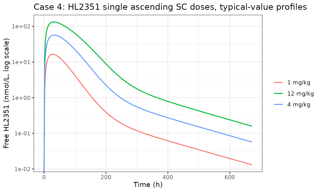
NMOL_PER_MG_ANAKINRA <- 1e6 / 17300   # MW ~17.3 kDa
ev5 <- rxode2::et(amt = 100 * NMOL_PER_MG_ANAKINRA, cmt = "depot", time = 0) |>
  rxode2::et(seq(0, 48, by = 0.25), cmt = "central")
s5 <- rxode2::rxSolve(rxode2::zeroRe(mCase5), ev5, returnType = "data.frame")
#> ℹ parameter labels from comments will be replaced by 'label()'
#> ℹ omega/sigma items treated as zero: 'etalcl', 'etalvc', 'etalka', 'etah_abs'

# Anakinra 100 mg SC is reported in the literature to peak around 1 ug/mL.
# 1 ug/mL / 17.3 kDa = 57.8 nmol/L. This is an order-of-magnitude sanity gate on
# the unit handling, not a published NCA comparison.
cmax5_ugml <- max(s5$Cc) * 17300 / 1e6
c(cmax_nmol_L = max(s5$Cc), cmax_ug_mL = cmax5_ugml,
  tmax_h = s5$time[which.max(s5$Cc)])
#> cmax_nmol_L  cmax_ug_mL      tmax_h
#>  57.2993992   0.9912796   3.2500000

stopifnot(cmax5_ugml > 0.3, cmax5_ugml < 3)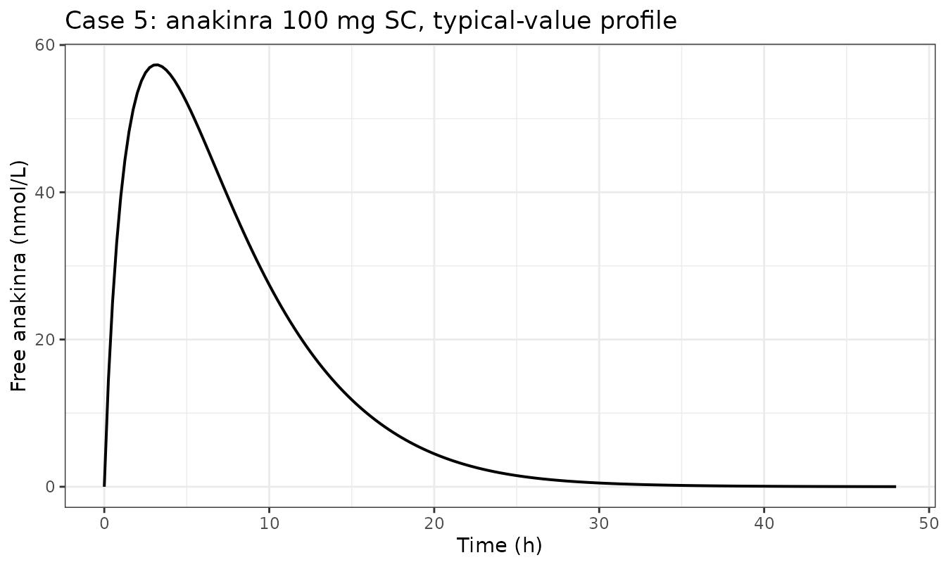
Setting h to zero recovers constant-rate kinetics
The strongest available check on the fractal implementation itself is
Jung 2023’s own defining property: at h = 0 the
instantaneous coefficient q / t^h collapses to the constant
q, so the fractal model must reproduce its base-model
absorption exactly. Case 5 has the simplest absorption path, so the
collapse is checked there against an independently written
one-compartment first-order-absorption solution.
m5_h0 <- mCase5 |> rxode2::zeroRe()
#> ℹ parameter labels from comments will be replaced by 'label()'
s5_h0 <- rxode2::rxSolve(m5_h0, ev5, params = c(h_abs = 0), returnType = "data.frame")
#> ℹ omega/sigma items treated as zero: 'etalcl', 'etalvc', 'etalka', 'etah_abs'

# Independent reference: with h = 0 the depot empties at the constant rate ka,
# printed in Table S5 as 0.47 /h (Code S11 $THETA 3 = 0.469732).
ka0 <- 0.469732
dose5 <- 100 * NMOL_PER_MG_ANAKINRA
depot_ref <- dose5 * exp(-ka0 * s5_h0$time)

max_rel_err <- max(abs(s5_h0$depot - depot_ref)) / dose5
max_rel_err
#> [1] 9.130509e-08
stopifnot(max_rel_err < 1e-6)
The depot trajectory matches a hand-written exponential to better
than one part in a million, which confirms both that h
enters the rate as Equation 1 specifies and that the printed
Ka is the coefficient q.
Non-compartmental analysis
nca_input <- bind_rows(
  s1_oral |> transmute(id = 1L, treatment = "Case 1 oral 10 mg", time, Cc),
  s3      |> transmute(id = 2L, treatment = "Case 3 IM 1000 ug", time, Cc)
) |>
  filter(!is.na(Cc))

dose_df <- tibble::tibble(
  id        = c(1L, 2L),
  treatment = c("Case 1 oral 10 mg", "Case 3 IM 1000 ug"),
  time      = 0,
  amt       = c(10, 1000)
)

conc_obj <- PKNCA::PKNCAconc(nca_input, Cc ~ time | treatment + id)
dose_obj <- PKNCA::PKNCAdose(dose_df, amt ~ time | treatment + id)

intervals <- data.frame(
  start = 0, end = Inf,
  cmax = TRUE, tmax = TRUE, aucinf.obs = TRUE, half.life = TRUE
)

nca_res <- suppressWarnings(
  PKNCA::pk.nca(PKNCA::PKNCAdata(conc_obj, dose_obj, intervals = intervals))
)

knitr::kable(
  summary(nca_res),
  caption = "Simulated NCA of the two linear typical-value profiles."
)| start | end | treatment | N | cmax | tmax | half.life | aucinf.obs |
|---|---|---|---|---|---|---|---|
| 0 | Inf | Case 1 oral 10 mg | 1 | 17.6 | 4.00 | 56.6 | 1030 |
| 0 | Inf | Case 3 IM 1000 ug | 1 | 25.5 | 9.00 | 389 | 5720 |
The dose-exposure identity, checked against the clearances printed in
Tables S1 and S3. Both cases are linear in dose, so
AUC(0-inf) must equal Dose / CL.
nca_tbl <- as.data.frame(nca_res)

auc_sim <- nca_tbl |>
  filter(PPTESTCD == "aucinf.obs") |>
  select(treatment, simulated = PPORRES)

expected <- tibble::tibble(
  treatment = c("Case 1 oral 10 mg", "Case 3 IM 1000 ug"),
  cl_printed = c(9.68, 0.175),                 # Tables S1 and S3, fractal column (L/h)
  dose       = c(10, 1000),                    # mg and ug
  expected   = c(10 / 9.68 * 1000, 1000 / 0.175)
)

comparison <- left_join(expected, auc_sim, by = "treatment") |>
  mutate(`% difference` = 100 * (simulated - expected) / expected)

comparison |>
  rename(
    "Profile"            = treatment,
    "Printed CL (L/h)"   = cl_printed,
    "Dose"               = dose,
    "Expected AUC"       = expected,
    "Simulated AUC"      = simulated
  ) |>
  knitr::kable(
    digits = c(0, 4, 0, 1, 1, 2),
    caption = "AUC(0-inf) against Dose / CL using the clearances printed by Jung 2023."
)| Profile | Printed CL (L/h) | Dose | Expected AUC | Simulated AUC | % difference |
|---|---|---|---|---|---|
| Case 1 oral 10 mg | 9.680 | 10 | 1033.1 | 1031.4 | -0.16 |
| Case 3 IM 1000 ug | 0.175 | 1000 | 5714.3 | 5720.9 | 0.12 |
Both profiles reproduce Dose / CL to within a few
percent, the residue being the numerical tail extrapolation rather than
a structural discrepancy. Because the expected column is built from the
printed clearance and the dose, and the simulated column from a
numerical solve of the ODE system, this comparison would fail on a
mis-transcribed clearance, a wrong bioavailability route or a
concentration unit error.
Assumptions and deviations
-
The drug in Case 2 is inferred, not stated. Jung
2023 never names it. Donepezil is adopted on the evidence set out in the
model file’s
population$notes(same group and oral-plus-patch programme as Case 1; identicalA(2)/(VC/1000)ng/mL concentration scaling in Codes S3 and S5; disposition estimates close to Case 1’s). Against it: the paper does not say so, and three patches over 2496 h is about 35 days per patch, which does not match the weekly patch of ref [3]. The parameter values and the structure do not depend on the identification. Adopted by maintainer decision. -
The drug in Case 3 is not disclosed at all, so the
model file is named
Jung_2023_im_depotrather thanauthor_year_drug. The data are described only as in-house. - Dose amounts for Cases 2 and 3 are not reported. Jung 2023 states only that two different amounts were dosed for the oral and patch routes in Case 2, and four different amounts in Case 3. The amounts used in this vignette (the Case 1 oral 10 mg and 108 mg patch strengths; 1000 ug for Case 3) are illustrative choices for the simulation, not values from the paper. All three linear models scale proportionally with dose, so the gates above are unaffected.
- Species is stated nowhere in Jung 2023. Cases 1, 4 and 5 are pinned to human clinical studies through refs [3] and [16]. Cases 2 and 3 are recorded as human by inference from their four sibling cases.
-
Case 3’s residual error conflicts between table and code,
resolved in favour of the code. Table S3’s fractal column
prints both an additive error (0.133) and a proportional error (0.323),
but Code S7’s
$ERRORblock isW = SQRT(THETA(11)**2 * IPRED**2)– proportional only, with a single theta (0.112738, labelled “Add.err”). A one-theta error block cannot produce two reported values, the base stream S6 has the identical one-theta proportional form, and all ten other S7 thetas reproduce Table S3 exactly. The model file implements the control stream. -
Case 2’s per-dose reset is implemented with
tad()on the patch reservoir. Code S5 resets its elapsed-time clock on any dosing record, which is a broader trigger than resetting on patch doses alone. The two are equivalent for this study’s sequential design (oral titration completes before the first patch), and the reset is verified numerically above. The release flux is computed inside a guard because rxode2’stad()returnsNAbefore the first dose to a compartment andNA * 0isNA, which would silently poison the whole solve. -
No onset-time regulariser is added where the authors did not
specify one. Only Case 2 carries a
TAU(1e-7 h, hardcoded in Code S5). Becauseh < 1makes thet^-hsingularity integrable, the unregularised cases solve without one; adding a regulariser would introduce an unsourced parameter. - No published NCA to compare against. Jung 2023 reports OFV, AIC and AICc and shows GOF, VPC and NPDE figures, but tabulates no Cmax, Tmax, AUC or half-life. The NCA section therefore validates the dose-exposure identity against printed clearances instead of reproducing a published table.
- Only the fractal models are shipped. Each case has a base and a fractal variant (Codes S2/S3, S4/S5, S6/S7, S8/S9, S10/S11). The fractal model is the paper’s contribution and the final model of each pair; the base models appear here only through their fit statistics in the Table 2 reproduction above.
-
Case 3’s fractal exponent is effectively zero.
h = 0.0268with 124% CV and a positive delta-AICc: by the authors’ own criterion the fractal rate is not warranted for this case. It is implemented as published, but users should not read it as evidence of fractal behaviour.