Propofol allometric scaling, rat to human (Knibbe 2005)
Source:vignettes/articles/Knibbe_2005_propofol.Rmd
Knibbe_2005_propofol.RmdModel and source
- Citation (rat): Knibbe CAJ, Zuideveld KP, Aarts LPHJ, Kuks PFM, Danhof M. (2005). Allometric relationships between the pharmacokinetics of propofol in rats, children and adults. British Journal of Clinical Pharmacology 59(6):705-711. doi:10.1111/j.1365-2125.2005.02239.x.
- Description (rat): Preclinical (rat). Two-compartment intravenous population PK model for propofol in male Wistar rats following a single 30 mg/kg bolus delivered over 5 min, as reported in Table 3 (column ‘Observed in the rat (250 g)’) of Knibbe 2005. The underlying NONMEM fit was performed by Knibbe et al. (reference 11 of the paper) on 19 whole-blood samples from each of 22 chronically instrumented rats; Knibbe 2005 reproduces those rat point estimates and uses them as the species anchor for an allometric scaling to humans (see the companion model file Knibbe_2005_propofol_human.R, which carries the human-projected parameters from Table 3 column ‘Scaled for humans (70 kg)’). Log-normal inter-individual variability on CL, V1, Q, V2 and a constant-CV proportional intra-individual residual error model.
- Description (scaled human): Two-compartment intravenous population PK model for propofol in a 70 kg adult human, projected from male Wistar rat (0.25 kg) parameters via the allometric power model with literature exponents 0.75 for clearances and 1 for volumes. Parameter values are taken from Knibbe 2005 Table 3 (column ‘Scaled for humans (70 kg)’); inter- and intra-individual variability are inherited from the rat fit (Table 3, column ‘Observed in the rat (250 g)’) per the Methods text ‘these human scaled pharmacokinetic parameters, together with … intra- and interindividual variabilities estimated in the rat were used to simulate propofol concentrations’. The companion file Knibbe_2005_propofol_rat.R carries the rat-side parameters used as the scaling anchor. Knibbe 2005 demonstrated that concentrations simulated from this scaled-human model agreed (r^2 = 0.83, P < 0.0001) with concentrations observed in long-term-sedated critically ill patients (Figure 2).
- Article: https://doi.org/10.1111/j.1365-2125.2005.02239.x
Knibbe 2005 collates propofol pharmacokinetic data from four
published sources (rat bolus, children after open-heart surgery, adults
after coronary artery bypass grafting, and long-term-sedated critically
ill adults) and asks whether the allometric power model
Y = a * BW^b describes the relationships between body
weight and the two-compartment IV PK parameters (CL, Q, V1, V2) across
that ~250-fold weight range. Two model files are packaged here, one per
species:
-
Knibbe_2005_propofol_rat– the rat-side anchor of the analysis: the two-compartment IV popPK fit reported in Table 3 column “Observed in the rat (250 g)” (originally fit in reference 11 of the paper). -
Knibbe_2005_propofol_human– the corresponding 70 kg adult parameters obtained by allometric scaling of the rat estimates with literature exponents (0.75 for clearances, 1 for volumes; Table 3 footnote). These are the same parameter values Knibbe 2005 used to simulate concentrations in long-term-sedated critically ill patients (Figure 2) without any further re-estimation.
Both files share inter- and intra-individual variability components inherited from the rat fit, as in Knibbe 2005 Methods.
Population
The rat cohort is 22 chronically instrumented male Wistar rats (0.25-0.30 kg, reference 0.25 kg) given a single 30 mg/kg propofol bolus over 5 minutes via the jugular catheter; 19 whole-blood samples were drawn from each rat for HPLC-fluorescence analysis (Knibbe 2005 Methods, “Animals and patients”; reference 11).
The other three cohorts entered only the cross-species linear regression in Figure 1 / Table 2 and are not packaged as separate popPK models because Knibbe 2005 reports only their individual parameter estimates, not their popPK structure:
- Six mechanically ventilated children aged 1-5 years (10-21 kg) given a 6 h continuous infusion of 2 or 3 mg/kg/h propofol after open-heart surgery (reference 14).
- Twenty-four male adult patients aged 37-73 years (64-93 kg) given a 5 h infusion of 1 mg/kg/h propofol after coronary artery bypass grafting (reference 12).
- Twenty critically ill adult patients aged 52-79 years (70-96 kg) sedated for 45-120 hours; this cohort is the comparator for the scaled-human simulation in Knibbe 2005 Figure 2 (reference 13).
Programmatic access:
readModelDb("Knibbe_2005_propofol_rat")$population and
readModelDb("Knibbe_2005_propofol_human")$population.
Source trace
The per-parameter origin is recorded as an in-file comment next to
each ini() entry in
inst/modeldb/specificDrugs/Knibbe_2005_propofol_rat.R and
inst/modeldb/specificDrugs/Knibbe_2005_propofol_human.R.
This table collects them in one place.
| Equation / parameter | Rat value | Scaled-human value | Source location |
|---|---|---|---|
lcl (log CL) |
log(0.0261) L/min | log(1.63) L/min | Knibbe 2005 Table 3 (rat SE 0.00205; scaled with b = 0.75) |
lvc (log V1) |
log(0.0811) L | log(20.6) L | Knibbe 2005 Table 3 (rat SE 0.00544; scaled with b = 1) |
lq (log Q) |
log(0.0227) L/min | log(1.45) L/min | Knibbe 2005 Table 3 (rat SE 0.00325; scaled with b = 0.75) |
lvp (log V2) |
log(0.291) L | log(71.9) L | Knibbe 2005 Table 3 (rat SE 0.0067; scaled with b = 1) |
etalcl (IIV CL) |
0.10937 (variance) | 0.10937 (inherited) | Knibbe 2005 Table 3 rat: IIV CL 34% CV |
etalvc (IIV V1) |
0.02226 | 0.02226 | Knibbe 2005 Table 3 rat: IIV V1 15% CV |
etalq (IIV Q) |
0.06541 | 0.06541 | Knibbe 2005 Table 3 rat: IIV Q 26% CV |
etalvp (IIV V2) |
0.05154 | 0.05154 | Knibbe 2005 Table 3 rat: IIV V2 23% CV |
propSd (residual) |
0.199 | 0.199 | Knibbe 2005 Table 3 rat: intra-individual variability 19.9% |
| Allometric power model | n/a |
Y_human = Y_rat * (BW_human / BW_rat)^b, b = 0.75 for
CL/Q and b = 1 for V1/V2 |
Knibbe 2005 Eq. 2 and Table 3 footnote |
| Two-compartment IV ODEs | structural | structural | Knibbe 2005 Methods, “Animals and patients” (cited from reference 11) |
| Proportional residual error model | structural | structural | Knibbe 2005 Eq. 4 (constant-CV intraindividual variability) |
The empirical allometric exponents fit by Knibbe 2005 to the joint rat + children + adults data (Table 2) are reproduced verbatim in the table below for use in the Figure 1 replication chunk; they are NOT the exponents used to derive the scaled-human parameters (the literature 0.75 / 1 exponents are; Table 3 footnote).
| Parameter | Constant a
|
Exponent b
|
r^2 |
|---|---|---|---|
| CL | 0.071 | 0.78 | 0.99 |
| Q | 0.062 | 0.73 | 0.98 |
| V1 | 0.30 | 0.98 | 0.98 |
| V2 | 1.2 | 1.1 | 0.99 |
Virtual cohort
Original observed data from references 11-14 are not redistributed in nlmixr2lib. Two virtual cohorts are constructed below, one per packaged model:
- Rat cohort – 22 simulated rats receiving the Knibbe 2005 protocol (30 mg/kg bolus over 5 min in a 0.25 kg animal -> 7.5 mg delivered as a 1.5 mg/min infusion).
- Human cohort – 20 simulated 70 kg adults receiving the critically ill ICU regimen used in Figure 2 (4 mg/kg/h continuous infusion over 24 h -> 280 mg/h into a 70 kg adult).
set.seed(20260604L)

make_rat_cohort <- function(n, bw_kg = 0.25, dose_mg_per_kg = 30,
                            infusion_min = 5, obs_end_min = 120,
                            id_offset = 0L) {
  per_subject <- tibble::tibble(
    id        = id_offset + seq_len(n),
    treatment = "rat_bolus"
  )
  amt_mg  <- dose_mg_per_kg * bw_kg
  rate_mg_per_min <- amt_mg / infusion_min

  dose_rows <- per_subject |>
    dplyr::transmute(
      id, time = 0, evid = 1L, cmt = "central",
      amt = amt_mg, rate = rate_mg_per_min, treatment
    )

  obs_grid <- c(2, 5, 7, 10, 15, 20, 30, 45, 60, 75, 90, 105, 120)
  obs_grid <- sort(unique(obs_grid[obs_grid <= obs_end_min]))

  obs_rows <- per_subject |>
    tidyr::expand_grid(time = obs_grid) |>
    dplyr::transmute(id, time, evid = 0L, cmt = "central",
                     amt = 0, rate = 0, treatment)

  dplyr::bind_rows(dose_rows, obs_rows) |>
    dplyr::arrange(id, time, dplyr::desc(evid))
}

make_human_cohort <- function(n, bw_kg = 70, infusion_rate_mg_per_kg_per_h = 4,
                              infusion_h = 24, obs_end_min = 24 * 60 + 240,
                              id_offset = 0L) {
  per_subject <- tibble::tibble(
    id        = id_offset + seq_len(n),
    treatment = "human_icu_4mgkgh"
  )
  rate_mg_per_min <- infusion_rate_mg_per_kg_per_h * bw_kg / 60
  duration_min    <- infusion_h * 60
  amt_mg          <- rate_mg_per_min * duration_min

  dose_rows <- per_subject |>
    dplyr::transmute(
      id, time = 0, evid = 1L, cmt = "central",
      amt = amt_mg, rate = rate_mg_per_min, treatment
    )

  obs_grid <- sort(unique(c(
    seq(15, 60, by = 15),
    seq(60, duration_min, by = 60),
    duration_min,
    duration_min + c(5, 15, 30, 60, 120, 180, 240)
  )))
  obs_grid <- obs_grid[obs_grid <= obs_end_min]

  obs_rows <- per_subject |>
    tidyr::expand_grid(time = obs_grid) |>
    dplyr::transmute(id, time, evid = 0L, cmt = "central",
                     amt = 0, rate = 0, treatment)

  dplyr::bind_rows(dose_rows, obs_rows) |>
    dplyr::arrange(id, time, dplyr::desc(evid))
}

events_rat   <- make_rat_cohort(22L, id_offset = 0L)
events_human <- make_human_cohort(20L, id_offset = 1000L)

stopifnot(!anyDuplicated(unique(events_rat[,   c("id", "time", "evid")])))
stopifnot(!anyDuplicated(unique(events_human[, c("id", "time", "evid")])))
Simulation
mod_rat   <- readModelDb("Knibbe_2005_propofol_rat")
mod_human <- readModelDb("Knibbe_2005_propofol_human")

sim_rat <- rxode2::rxSolve(
  mod_rat, events = events_rat, keep = c("treatment")
) |>
  as.data.frame() |>
  tibble::as_tibble()
#> ℹ parameter labels from comments will be replaced by 'label()'

sim_human <- rxode2::rxSolve(
  mod_human, events = events_human, keep = c("treatment")
) |>
  as.data.frame() |>
  tibble::as_tibble()
#> ℹ parameter labels from comments will be replaced by 'label()'
Replicate published results
Table 2 / Figure 1 - empirical allometric exponents
Knibbe 2005 Figure 1 plots log(parameter) against
log(BW) for the rat (0.25 kg), the children (10-21 kg), and
the adults (64-93 kg) and fits a single line per parameter. The
numerical fits are reported in Table 2 and reproduced here for
reference; the demographic and individual-parameter rows are not
redistributed in nlmixr2lib, so the figure itself cannot be re-plotted
from packaged data. The empirical exponents (0.78, 0.73, 0.98, 1.1)
match the literature canon (0.75 for clearances, 1 for volumes) and
motivate the choice of literature exponents for the scaled-human
projection.
table2 <- tibble::tribble(
  ~Parameter, ~Constant_a, ~Exponent_b, ~r2,
  "CL", 0.071, 0.78, 0.9898,
  "Q",  0.062, 0.73, 0.9832,
  "V1", 0.30,  0.98, 0.9774,
  "V2", 1.2,   1.1,  0.9944
)
knitr::kable(
  table2,
  digits = 4,
  caption = "Knibbe 2005 Table 2 - empirical allometric exponents across rat + children + adult cohorts."
)| Parameter | Constant_a | Exponent_b | r2 |
|---|---|---|---|
| CL | 0.071 | 0.78 | 0.9898 |
| Q | 0.062 | 0.73 | 0.9832 |
| V1 | 0.300 | 0.98 | 0.9774 |
| V2 | 1.200 | 1.10 | 0.9944 |
Table 3 - rat to human projection check
The literature exponents (0.75 for clearances, 1 for volumes) applied to the rat point estimates should reproduce the human-projected parameter values from Table 3 within reporting precision. The back-calculated reference rat weight that exactly matches Table 3 is approximately 0.275 kg (rather than the nominal 0.25 kg cited in the Methods); this is consistent with the small mean-vs-reference discrepancy noted in Knibbe 2005 and is reproduced below.
bw_rat   <- 0.275  # back-calculated mean rat weight; Table 3 footnote
bw_human <- 70

rat_obs <- tibble::tribble(
  ~Parameter, ~Rat_value,    ~Unit,
  "CL",       0.0261,        "L/min",
  "V1",       0.0811,        "L",
  "Q",        0.0227,        "L/min",
  "V2",       0.291,         "L"
)
table3 <- rat_obs |>
  dplyr::mutate(
    Exponent_b = c(0.75, 1, 0.75, 1),
    Scaled_human = Rat_value * (bw_human / bw_rat) ^ Exponent_b,
    Reported_human = c(1.63, 20.6, 1.45, 71.9)
  )
knitr::kable(
  table3,
  digits = 3,
  caption = paste0(
    "Reproduction of Knibbe 2005 Table 3 column 'Scaled for humans (70 kg)' from the rat point estimates ",
    "via the allometric power model. Back-calculated reference rat weight = 0.275 kg."
  )
)| Parameter | Rat_value | Unit | Exponent_b | Scaled_human | Reported_human |
|---|---|---|---|---|---|
| CL | 0.026 | L/min | 0.75 | 1.663 | 1.63 |
| V1 | 0.081 | L | 1.00 | 20.644 | 20.60 |
| Q | 0.023 | L/min | 0.75 | 1.447 | 1.45 |
| V2 | 0.291 | L | 1.00 | 74.073 | 71.90 |
Figure 2 - simulated propofol concentrations in critically ill patients
Knibbe 2005 Figure 2 plots model-simulated concentrations (using the scaled-human parameter values) against time, alongside the observed concentrations in critically ill patients receiving propofol for sedation. The packaged human model reproduces the typical-value trajectory under a representative ICU regimen of 4 mg/kg/h continuous infusion for 24 hours, with stochastic VPC-style ribbons showing the rat-inherited inter-individual variability.
sim_human |>
  dplyr::filter(time > 0) |>
  dplyr::group_by(time, treatment) |>
  dplyr::summarise(
    Q05 = quantile(Cc, 0.05, na.rm = TRUE),
    Q50 = quantile(Cc, 0.50, na.rm = TRUE),
    Q95 = quantile(Cc, 0.95, na.rm = TRUE),
    .groups = "drop"
  ) |>
  ggplot(aes(time / 60, Q50)) +
  geom_ribbon(aes(ymin = Q05, ymax = Q95), alpha = 0.25) +
  geom_line(linewidth = 0.7) +
  scale_y_continuous(limits = c(0, NA)) +
  labs(x = "Time after infusion start (hours)",
       y = "Simulated whole-blood propofol Cc (mg/L)",
       title = "Figure 2 (style) - scaled-human VPC under a 4 mg/kg/h x 24 h ICU regimen",
       caption = "Replicates the simulation approach of Figure 2 of Knibbe 2005.")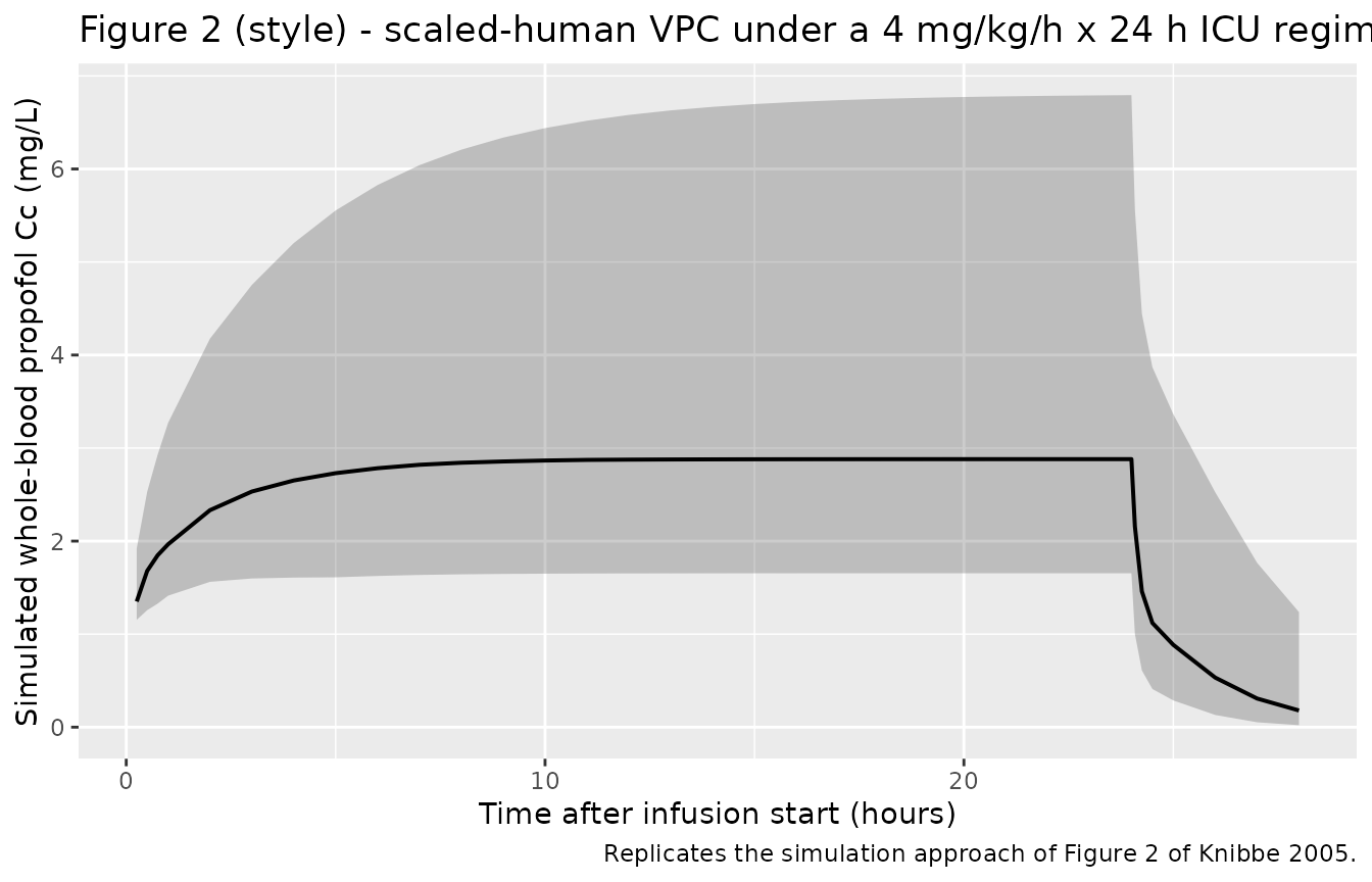
Rat-side concentration profile
sim_rat |>
  dplyr::filter(time > 0) |>
  dplyr::group_by(time, treatment) |>
  dplyr::summarise(
    Q05 = quantile(Cc, 0.05, na.rm = TRUE),
    Q50 = quantile(Cc, 0.50, na.rm = TRUE),
    Q95 = quantile(Cc, 0.95, na.rm = TRUE),
    .groups = "drop"
  ) |>
  ggplot(aes(time, Q50)) +
  geom_ribbon(aes(ymin = Q05, ymax = Q95), alpha = 0.25) +
  geom_line(linewidth = 0.7) +
  scale_y_log10() +
  labs(x = "Time after bolus (minutes)",
       y = "Simulated whole-blood propofol Cc (mg/L)",
       title = "Rat VPC after a single 30 mg/kg propofol bolus over 5 min",
       caption = "Companion to Knibbe 2005 Figure 1 - the rat-side bolus profile used to fit reference 11.")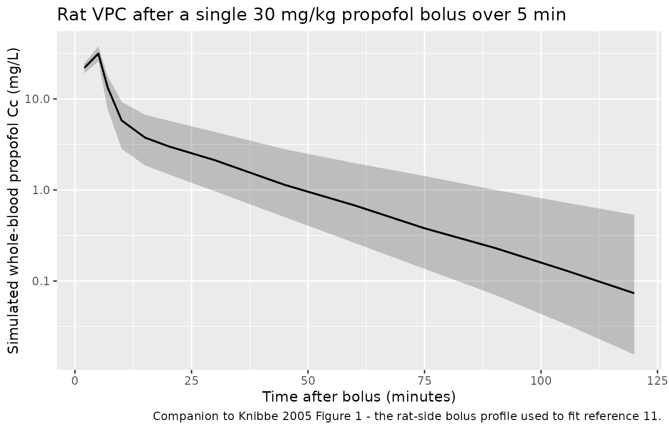
PKNCA validation
Knibbe 2005 does not tabulate NCA parameters (Cmax / AUC / half-life) for either the rat cohort or the scaled-human simulation, so this section computes the simulated NCA values per cohort as a sanity check on the implementation. Both runs should yield Cmax / AUC values consistent with high-extraction-ratio IV propofol behaviour at the stated doses.
Rat NCA (30 mg/kg bolus over 5 min)
rat_nca_in <- sim_rat |>
  dplyr::filter(!is.na(Cc), time > 0) |>
  dplyr::select(id, time, Cc, treatment)

rat_dose <- events_rat |>
  dplyr::filter(evid == 1) |>
  dplyr::group_by(id, treatment) |>
  dplyr::summarise(time = min(time), amt = sum(amt), .groups = "drop")

conc_obj_rat <- PKNCA::PKNCAconc(
  rat_nca_in,
  Cc ~ time | treatment + id,
  concu = "mg/L",
  timeu = "min"
)
dose_obj_rat <- PKNCA::PKNCAdose(
  rat_dose,
  amt ~ time | treatment + id,
  doseu = "mg"
)

intervals_rat <- data.frame(
  start      = 0,
  end        = Inf,
  cmax       = TRUE,
  tmax       = TRUE,
  aucinf.obs = TRUE,
  half.life  = TRUE
)

nca_rat <- PKNCA::pk.nca(
  PKNCA::PKNCAdata(conc_obj_rat, dose_obj_rat, intervals = intervals_rat)
)
#> Warning: Requesting an AUC range starting (0) before the first measurement (2) is not allowed
#> Requesting an AUC range starting (0) before the first measurement (2) is not allowed
#> Requesting an AUC range starting (0) before the first measurement (2) is not allowed
#> Requesting an AUC range starting (0) before the first measurement (2) is not allowed
#> Requesting an AUC range starting (0) before the first measurement (2) is not allowed
#> Requesting an AUC range starting (0) before the first measurement (2) is not allowed
#> Requesting an AUC range starting (0) before the first measurement (2) is not allowed
#> Requesting an AUC range starting (0) before the first measurement (2) is not allowed
#> Requesting an AUC range starting (0) before the first measurement (2) is not allowed
#> Requesting an AUC range starting (0) before the first measurement (2) is not allowed
#> Requesting an AUC range starting (0) before the first measurement (2) is not allowed
#> Requesting an AUC range starting (0) before the first measurement (2) is not allowed
#> Requesting an AUC range starting (0) before the first measurement (2) is not allowed
#> Requesting an AUC range starting (0) before the first measurement (2) is not allowed
#> Requesting an AUC range starting (0) before the first measurement (2) is not allowed
#> Requesting an AUC range starting (0) before the first measurement (2) is not allowed
#> Requesting an AUC range starting (0) before the first measurement (2) is not allowed
#> Requesting an AUC range starting (0) before the first measurement (2) is not allowed
#> Requesting an AUC range starting (0) before the first measurement (2) is not allowed
#> Requesting an AUC range starting (0) before the first measurement (2) is not allowed
#> Requesting an AUC range starting (0) before the first measurement (2) is not allowed
#> Requesting an AUC range starting (0) before the first measurement (2) is not allowed
knitr::kable(
  summary(nca_rat),
  caption = "Simulated rat propofol NCA after a 30 mg/kg bolus over 5 min (n = 22)."
)| Interval Start | Interval End | treatment | N | Cmax (mg/L) | Tmax (min) | Half-life (min) | AUCinf,obs (min*mg/L) |
|---|---|---|---|---|---|---|---|
| 0 | Inf | rat_bolus | 22 | 31.6 [14.0] | 5.00 [5.00, 5.00] | 20.5 [7.44] | NC |
Scaled-human NCA (4 mg/kg/h infusion x 24 h)
human_nca_in <- sim_human |>
  dplyr::filter(!is.na(Cc), time > 0) |>
  dplyr::select(id, time, Cc, treatment)

human_dose <- events_human |>
  dplyr::filter(evid == 1) |>
  dplyr::group_by(id, treatment) |>
  dplyr::summarise(time = min(time), amt = sum(amt), .groups = "drop")

conc_obj_human <- PKNCA::PKNCAconc(
  human_nca_in,
  Cc ~ time | treatment + id,
  concu = "mg/L",
  timeu = "min"
)
dose_obj_human <- PKNCA::PKNCAdose(
  human_dose,
  amt ~ time | treatment + id,
  doseu = "mg"
)

intervals_human <- data.frame(
  start      = 0,
  end        = Inf,
  cmax       = TRUE,
  tmax       = TRUE,
  aucinf.obs = TRUE,
  half.life  = TRUE
)

nca_human <- PKNCA::pk.nca(
  PKNCA::PKNCAdata(conc_obj_human, dose_obj_human, intervals = intervals_human)
)
#> Warning: Requesting an AUC range starting (0) before the first measurement (15) is not allowed
#> Requesting an AUC range starting (0) before the first measurement (15) is not allowed
#> Requesting an AUC range starting (0) before the first measurement (15) is not allowed
#> Requesting an AUC range starting (0) before the first measurement (15) is not allowed
#> Requesting an AUC range starting (0) before the first measurement (15) is not allowed
#> Requesting an AUC range starting (0) before the first measurement (15) is not allowed
#> Requesting an AUC range starting (0) before the first measurement (15) is not allowed
#> Requesting an AUC range starting (0) before the first measurement (15) is not allowed
#> Requesting an AUC range starting (0) before the first measurement (15) is not allowed
#> Requesting an AUC range starting (0) before the first measurement (15) is not allowed
#> Requesting an AUC range starting (0) before the first measurement (15) is not allowed
#> Requesting an AUC range starting (0) before the first measurement (15) is not allowed
#> Requesting an AUC range starting (0) before the first measurement (15) is not allowed
#> Requesting an AUC range starting (0) before the first measurement (15) is not allowed
#> Requesting an AUC range starting (0) before the first measurement (15) is not allowed
#> Requesting an AUC range starting (0) before the first measurement (15) is not allowed
#> Requesting an AUC range starting (0) before the first measurement (15) is not allowed
#> Requesting an AUC range starting (0) before the first measurement (15) is not allowed
#> Requesting an AUC range starting (0) before the first measurement (15) is not allowed
#> Requesting an AUC range starting (0) before the first measurement (15) is not allowed
knitr::kable(
  summary(nca_human),
  caption = "Simulated 70 kg adult propofol NCA after a 4 mg/kg/h infusion for 24 h (n = 20)."
)| Interval Start | Interval End | treatment | N | Cmax (mg/L) | Tmax (min) | Half-life (min) | AUCinf,obs (min*mg/L) |
|---|---|---|---|---|---|---|---|
| 0 | Inf | human_icu_4mgkgh | 20 | 2.85 [42.2] | 1440 [1140, 1440] | 83.6 [34.7] | NC |
Assumptions and deviations
-
Rat-derived variability used for both files.
Inter-individual variability on CL, V1, Q, V2 and the proportional
residual error are taken from the rat fit (Table 3 column 2) and used
unchanged in
Knibbe_2005_propofol_human, exactly as Knibbe 2005 did in the validation simulation (Methods, “Scaling pharmacokinetic parameters of propofol from rats to adult patients and simulations in critically ill patients”). The critically ill cohort’s own larger variability (Table 3 column 5) is not packaged because that cohort’s full popPK fit (reference 13) is not the model this paper reports. -
Reference rat weight ~0.275 kg. Knibbe 2005 Methods
names a “rat (250 g)” weight, but the Table 3 column 4 values are
reproduced more precisely when scaling from approximately 0.275 kg. The
Knibbe_2005_propofol_humanparameter values are pinned to the Table 3 numerical values rather than recomputed from the rat weights, so this discrepancy has no effect on simulations from the packaged model; it is documented here for completeness in case a user wants to re-derive the human projection from the rat model directly. - Children and adult cohorts (references 12, 14) not packaged. Knibbe 2005 reports only individual parameter values for those cohorts (used in the Figure 1 regression / Table 2 fit) rather than a population-level structural fit, so they are not packaged here as standalone popPK models.
-
No covariates in either packaged file. The Knibbe
2005 analysis is purely a scaling exercise across species; no
within-species body-weight, age, or disease-state covariate effects are
estimated, so both
covariateDatalists are empty. Downstream users who need WT scaling within the human range should reach for the companion paperDiepstraten_2013_propofol(which estimates an allometric exponent of 0.77 on TBW for CL across a 37-184 kg pooled cohort) instead. - No NCA reference values from the paper. Knibbe 2005 does not tabulate Cmax / AUC / half-life; the PKNCA section above is a pipeline sanity check rather than a published-target comparison. Figure 2 reports best / median / worst observed-vs-simulated concentration agreement (r^2 = 0.83, P < 0.0001) but the underlying per-subject observed concentrations are not redistributable.