Vincristine and peripheral neuropathy (Centanni 2024)
Source:vignettes/articles/Centanni_2024_vincristine.Rmd
Centanni_2024_vincristine.RmdModel and source
- Citation: Centanni M, van de Velde ME, Uittenboogaard A, Kaspers GJL, Karlsson MO, Friberg LE. Model-Informed Precision Dosing to Reduce Vincristine-Induced Peripheral Neuropathy in Pediatric Patients: A Pharmacokinetic and Pharmacodynamic Modeling and Simulation Analysis. Clin Pharmacokinet. 2024;63(2):197-209. doi:10.1007/s40262-023-01336-1
- Description: Two-compartment population PK model for intravenous vincristine in children with cancer, linked to a proportional-odds Markov model for vincristine-induced peripheral neuropathy (VIPN; Centanni 2024, final estimated models of Tables 2 and 3). Linear disposition with allometric weight scaling (exponents fixed at 0.75 and 1, 70 kg reference), an infusion-only lag time and a multiplier on the documented infusion duration; log-additive residual error with separate magnitudes for bolus and infusion samples and IIV on the infusion residual. The neuropathy model gives the probability of CTCAE grade >= 1 and >= 2 for each of four subscores (sensory, motor, constipation, neuralgia) at each dosing occasion, driven by an Emax function of the occasion AUC = dose / CL, with a higher-risk intercept from the second occasion and a Markov term for a previous subscore above grade 0.
- Simulation variant: Simulation variant of the Centanni 2024 vincristine PK and neuropathy model for children with cancer, as used for the paper’s precision-dosing trial: clearance of the Table 2 two-compartment model replaced by the two-group CYP3A5 mixture (42.3 L/h at 70 kg, 1.87-fold higher in the 10% high expressers) with 32.3% IIV and 36.3% inter-occasion variability (one occasion per dose); all other parameters as in Centanni_2024_vincristine. Linear disposition with allometric weight scaling (exponents fixed at 0.75 and 1, 70 kg reference), an infusion-only lag time and a multiplier on the documented infusion duration; log-additive residual error with separate magnitudes for bolus and infusion samples and IIV on the infusion residual. The neuropathy model gives the probability of CTCAE grade >= 1 and >= 2 for each of four subscores (sensory, motor, constipation, neuralgia) at each dosing occasion, driven by an Emax function of the occasion AUC = dose / CL, with a higher-risk intercept from the second occasion and a Markov term for a previous subscore above grade 0.
- Article: https://doi.org/10.1007/s40262-023-01336-1 (open access)
Centanni et al. re-analysed the vincristine concentrations of the
randomized bolus-versus-infusion trial of van de Velde et al. 2020 (see
vandeVelde_2020_vincristine) and linked them to the CTCAE
grades of vincristine-induced peripheral neuropathy (VIPN) recorded
after every dose. The paper contributes two model files:
-
Centanni_2024_vincristine– the final estimated models: the PK model of Table 2 and the VIPN model of Table 3. Each dosing occasion was a separate individual when the PK model was fitted, so the 76.6% IIV on CL also carries the occasion-to-occasion variability. -
Centanni_2024_vincristine_mipd– the same model with the CL terms of the paper’s second-stage estimation, which split the per-occasion CL estimates into IIV (32.3%) and inter-occasion variability (36.3%) and fitted a two-group CYP3A5 mixture (42.3 L/h/70 kg in 90% of patients, 1.87-fold higher in 10%). The paper used it to generate the true exposures of its precision-dosing simulations (Table 4, Figures 3-5).
The PK model is two-compartmental with allometric weight scaling. The infusion arm has a lag time from bag to bloodstream and an infusion that lasts 1.30 times the documented duration (flushing), and its samples carry a larger residual error with IIV. The VIPN model is a proportional-odds model with a Markov element, applied to each of four CTCAE subscores (peripheral sensory neuropathy, peripheral motor neuropathy, constipation, neuralgia) on three levels (grade 0, 1, >= 2):
logit P(grade >= 1) = B1 + Emax x AUC / (AUC50 + AUC) + B>0 x [previous grade > 0]logit P(grade >= 2) = logit P(grade >= 1) + B2-
B1isB1|0on the first dosing occasion andB1|0, if OCC > 1from the second;B2is shared by neuralgia and motor neuropathy and by constipation and sensory neuropathy (Table 3). -
AUC = dose / CLof the current occasion, in ng*h/mL.
The model outputs p_vipn_ge1 (all subscores),
p_vipn_ge2_nm (neuralgia and motor) and
p_vipn_ge2_cs (constipation and sensory). The Markov state
enters through the PREV_AE_SCORE covariate, the occasion
through CYCLE. A later analysis by the same group (Centanni
et al. 2026, CPT Pharmacometrics Syst Pharmacol, doi:10.1002/psp4.70303)
re-estimated a related model and printed its NONMEM code; that code
builds the logits the same way (grade >= 2 logit = grade >= 1
logit + increment, previous-grade term inside the grade >= 1 logit,
constipation and sensory sharing one increment), which supports the
reading above.
Population
Table 1 describes 35 children (median age 9 years, range 2-17; median weight 34 kg, range 12-95; median BSA 1.2 m^2, range 0.5-2.2; 16 male). 64% were treated for acute lymphoblastic leukemia (ALL). Twenty were randomized to an IV bolus and fifteen to an infusion (standard 60 min of which 38 min of drug and 22 min of flushing; 96 min in four and 15 min in two patients). Doses were 1.5 or 2 mg/m^2 capped at 2 mg, over one to five occasions. Blood was sampled at 10, 20, 30, 40, 60, 75 and 140 min and at 24 h when still in hospital; 425 concentrations and 276 VIPN assessments were analysed.
The same information is available programmatically via
readModelDb("Centanni_2024_vincristine")()$population.
Source trace
The per-parameter origin is recorded as an in-file comment next to
each ini() entry in
inst/modeldb/specificDrugs/Centanni_2024_vincristine.R and
Centanni_2024_vincristine_mipd.R. The table below collects
them.
| Equation / parameter | Value | Source location |
|---|---|---|
lcl (estimation model) |
log(45.2) L/h at 70 kg | Table 2 CL |
lcl (_mipd) |
log(42.3) L/h at 70 kg | Results ‘Pharmacokinetic Model’ (90% group) |
e_cyp3a5_expr_cl (_mipd) |
1.87, fixed | Methods ‘Approximation of Non-estimated Factors’ (79.1 / 42.3) |
lvc |
log(23.3) L | Table 2 Vc |
lq |
log(114) L/h | Table 2 Q |
lvp |
log(576) L | Table 2 Vp |
ltlag |
log(0.058) h | Table 2 LAGT (infusion only) |
tinf_mult |
1.30 | Table 2 INFT |
e_wt_cl, e_wt_vc
|
0.75, 1 (fixed), 70 kg | Methods ‘Pharmacokinetic Model’; Table 2 footnote a |
etalcl (estimation model) |
0.4617 (76.6%) | Table 2 IIV CL |
etalcl (_mipd) |
0.0992 (32.3%) | Results ‘Pharmacokinetic Model’ |
etalcl_oc1-etalcl_oc5
(_mipd) |
0.1238 (36.3%) | Results ‘Pharmacokinetic Model’ |
etalvc |
0.4782 (78.3%) | Table 2 IIV Vc |
etaltlag |
0.4016 (70.3%) | Table 2 IIV LAGT |
etaRUV |
0.0765 (28.2%) | Table 2 IIV RUV (infusion samples) |
expSd_bolus |
0.137 | Table 2 RUVadd,bolus (log scale) |
expSd_infusion |
0.204 | Table 2 RUVadd,infusion (log scale) |
b1_vipn |
-121 | Table 3 B1|0 |
b1_occ_vipn |
-119.54 | Table 3 B1|0, if OCC > 1 (-120), refined from Figure S6 |
b2b1_nm_vipn |
-1.22 | Table 3 B2|0 (neuropathy/motor) |
b2b1_cs_vipn |
-3.59 | Table 3 B2|0 (constipation/sensory) |
b_prev_vipn |
2.81 | Table 3 B > 0|Grade > 0 |
emax_vipn |
119 | Table 3 Emax |
auc50_vipn |
0.164 ng*h/mL | Table 3 prints 1.62; 0.164 from Figure S6 |
| Two-compartment ODEs, allometry | – | Methods and Results ‘Pharmacokinetic Model’ |
| Proportional-odds logits | – | Eqs. 2-5; Results ‘Pharmacodynamic Model’ |
| AUC = dose / CL | – | Results ‘Pharmacodynamic Model’; Methods Eq. 7 text |
| Omega from CV% | log(1 + CV^2) |
Table 2 footnote b |
Neuropathy model: Online Resource 2 (Figure S6)
Table 3 prints the two intercepts and Emax to three significant figures, but the model uses them only as a near-cancelling sum (-121 + 119), so the rounding moves the net logit by up to one unit. The paper’s Online Resource 2 (Figure S6) plots P(grade >= 1) and P(grade >= 2) against AUC for six scenarios, “calculated using the expit function and parameter estimates”. The maintainers traced the curves from the supplement’s image (neuralgia/motor increment) and fitted Eqs. 4-5 to them with Emax, AUC50 and the intercepts free. The fit returned Emax = 119.0, B > 0|Grade > 0 = 2.81, B2|0 = -1.21 and B1|0 + Emax = -2.01, all matching Table 3, plus an occasion > 1 intercept of -119.54 (Table 3: -120) and an AUC50 of 0.164 ng*h/mL, where Table 3 prints 1.62. The packaged model carries the refined intercept and AUC50 = 0.164.
The chunk below solves the packaged model on a grid of AUC values and
compares it with the traced points, and repeats the solve with the two
printed values (b1_occ_vipn = -120,
auc50_vipn = 1.62).
# Traced from Online Resource 2 (Figure S6), probabilities. Scenario codes:
# DRUG = first occasion, previous grade 0; OCC1 = occasion > 1; PDV =
# previous grade > 0. Grade 2 panel uses the neuralgia/motor increment.
traced <- tibble::tribble(
  ~scenario, ~auc, ~p_ge1, ~p_ge2,
  "DRUG",       10, 0.0185, 0.0058,
  "DRUG",       20, 0.0491, 0.0153,
  "DRUG",       40, 0.0750, 0.0240,
  "DRUG",       75, 0.0935, 0.0298,
  "DRUG",      200, 0.1083, 0.0349,
  "DRUG_OCC1",  10, 0.0787, 0.0247,
  "DRUG_OCC1",  20, 0.1824, 0.0618,
  "DRUG_OCC1",  40, 0.2639, 0.0960,
  "DRUG_OCC1",  75, 0.3102, 0.1171,
  "DRUG_OCC1", 200, 0.3454, 0.1345,
  "PDV",        10, 0.2500, 0.0902,
  "PDV",        20, 0.4630, 0.2029,
  "PDV",        40, 0.5806, 0.2909,
  "PDV",        75, 0.6343, 0.3396,
  "PDV",       200, 0.6694, 0.3760,
  "PDV_OCC1",   10, 0.5852, 0.2960,
  "PDV_OCC1",   20, 0.7870, 0.5229,
  "PDV_OCC1",   40, 0.8556, 0.6385,
  "PDV_OCC1",   75, 0.8806, 0.6880,
  "PDV_OCC1",  200, 0.8972, 0.7222
)

mod <- readModelDb("Centanni_2024_vincristine")
mod_typ <- rxode2::zeroRe(rxode2::rxode(mod))
#> ℹ parameter labels from comments will be replaced by 'label()'
#> Warning: some etas defaulted to non-mu referenced, possible parsing error: etaRUV
#> as a work-around try putting the mu-referenced expression on a simple line
#> Warning: No sigma parameters in the model
#> Warning: some etas defaulted to non-mu referenced, possible parsing error: etaRUV
#> as a work-around try putting the mu-referenced expression on a simple line

scen <- tibble::tribble(
  ~scenario,   ~CYCLE, ~PREV_AE_SCORE,
  "DRUG",           1, 0,
  "DRUG_OCC1",      2, 0,
  "PDV",            1, 1,
  "PDV_OCC1",       2, 1
)
# A 70 kg typical subject: AUC = dose / CL, so dose (mg) = AUC x 45.2 / 1000
auc_grid <- c(0.5, 1, 2, 5, seq(10, 250, by = 10))
s6_events <- tidyr::expand_grid(scen, auc = auc_grid) |>
  dplyr::mutate(id = dplyr::row_number())
s6_events <- dplyr::bind_rows(
  s6_events |> dplyr::mutate(time = 0, evid = 1L, amt = auc * 45.2 / 1000),
  s6_events |> dplyr::mutate(time = 24, evid = 0L, amt = 0)
) |>
  dplyr::mutate(cmt = "central", WT = 70, TINF = 0) |>
  dplyr::arrange(id, time)

solve_s6 <- function(params = NULL) {
  out <- rxode2::rxSolve(mod_typ, events = s6_events, params = params,
                         keep = c("scenario", "auc"), returnType = "data.frame")
  dplyr::select(out, scenario, auc, auc_occ, p_vipn_ge1, p_vipn_ge2_nm)
}
s6_model <- solve_s6()
#> ℹ omega/sigma items treated as zero: 'etalcl', 'etalvc', 'etaltlag', 'etaRUV'
#> Warning: multi-subject simulation without without 'omega'
s6_printed <- solve_s6(c(b1_occ_vipn = -120, auc50_vipn = 1.62))
#> ℹ omega/sigma items treated as zero: 'etalcl', 'etalvc', 'etaltlag', 'etaRUV'
#> Warning: multi-subject simulation without without 'omega'

# The model's AUC is dose / CL of the subject, as in the paper
stopifnot(max(abs(s6_model$auc_occ / s6_model$auc - 1)) < 1e-6)

cmp_s6 <- traced |>
  dplyr::inner_join(s6_model, by = c("scenario", "auc")) |>
  dplyr::inner_join(
    s6_printed |> dplyr::select(scenario, auc,
                                printed_ge1 = p_vipn_ge1,
                                printed_ge2 = p_vipn_ge2_nm),
    by = c("scenario", "auc")
  )
err_model <- max(abs(c(cmp_s6$p_vipn_ge1 - cmp_s6$p_ge1,
                       cmp_s6$p_vipn_ge2_nm - cmp_s6$p_ge2)))
err_printed <- max(abs(c(cmp_s6$printed_ge1 - cmp_s6$p_ge1,
                         cmp_s6$printed_ge2 - cmp_s6$p_ge2)))
c(packaged_model = err_model, printed_table3 = err_printed)
#> packaged_model printed_table3
#>    0.002384123    0.799448260
# Deterministic: same equations, no random draws. The packaged values
# reproduce the authors' curves to tracing precision; the printed values
# miss them by tens of percentage points.
stopifnot(err_model < 0.02, err_printed > 0.3)
# Replicates Online Resource 2 (Figure S6) of Centanni 2024
s6_long <- dplyr::bind_rows(
  s6_model |> dplyr::mutate(source = "Packaged model"),
  s6_printed |> dplyr::mutate(source = "Table 3 as printed")
) |>
  tidyr::pivot_longer(c(p_vipn_ge1, p_vipn_ge2_nm), names_to = "grade",
                      values_to = "p") |>
  dplyr::mutate(grade = ifelse(grade == "p_vipn_ge1", "Grade >= 1",
                               "Grade >= 2 (neuralgia/motor)"))
traced_long <- traced |>
  tidyr::pivot_longer(c(p_ge1, p_ge2), names_to = "grade", values_to = "p") |>
  dplyr::mutate(grade = ifelse(grade == "p_ge1", "Grade >= 1",
                               "Grade >= 2 (neuralgia/motor)"))
ggplot(s6_long, aes(auc, p, colour = scenario)) +
  geom_line(aes(linetype = source)) +
  geom_point(data = traced_long) +
  facet_wrap(~grade, ncol = 1) +
  labs(x = "AUC (ng*h/mL)", y = "Probability", colour = "Scenario",
       linetype = NULL,
       caption = paste0("Points: traced from Online Resource 2 (Figure S6).\n",
                        "Lines: packaged model and Table 3 as printed.")) +
  theme(legend.position = "bottom", legend.box = "vertical")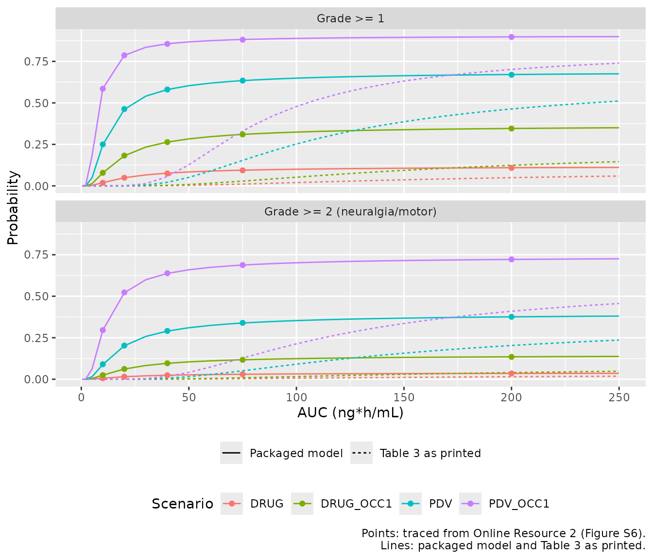
The printed AUC50 of 1.62 ng*h/mL is a factor of ten above the curves’ value; with it the model predicts almost no grade >= 2 VIPN at the protocol doses (see the Table 4 section below), against the 5.8% at the first occasion that the paper reports. The packaged value is 0.164.
Virtual cohorts
The observed data are not public. Two cohorts are used, both built in base R so that they are the same on every machine.
-
PK cohort (Table 1 population): weight log-normal
around the Table 1 median of 34 kg (SD of log 0.45), truncated to the
observed 12-95 kg; BSA from the weight-only Costeff formula
BSA = (4 WT + 7) / (WT + 90); one 1.5 mg/m^2 dose capped at 2 mg; 100 subjects as an IV bolus and 100 as the protocol 60-min infusion, entered as its 38 min of vincristine (TINF = 38/60; see the next section). - ALL cohort for the precision-dosing simulation (Methods ‘Generation of the Target Populations’): ages 1-18 years weighted towards the 2-5-year incidence peak of childhood ALL, weight from a log-linear interpolation of median weight against age (8.9 kg at 1 year, 11.5 kg at 2 years, 27.1 kg at 8.3 years and 70 kg at 18 years, the anchors of the Nijstad 2022 vincristine article) with 15% scatter, Costeff BSA, 1.5 mg/m^2 capped at 2 mg, high-clearance mixture group with probability 0.10; 200 subjects.
set.seed(20240201)
n_arm <- 100
pk_subjects <- tibble::tibble(
  id = seq_len(2 * n_arm),
  arm = rep(c("Bolus", "60-min infusion"), each = n_arm),
  TINF = rep(c(0, 38 / 60), each = n_arm),
  WT = pmin(pmax(34 * exp(rnorm(2 * n_arm, 0, 0.45)), 12), 95)
) |>
  dplyr::mutate(
    BSA = (4 * WT + 7) / (WT + 90),
    dose = pmin(1.5 * BSA, 2)
  )

obs_times <- c(0, 1 / 6, 1 / 3, 0.5, 2 / 3, 1, 1.25, 1.5, 2, 2.33, 3, 4, 6,
               8, 12, 24, 36, 48, 60, 72)
pk_events <- dplyr::bind_rows(
  pk_subjects |>
    dplyr::mutate(time = 0, evid = 1L, amt = dose,
                  rate = ifelse(TINF > 0, -2, 0)),
  tidyr::expand_grid(pk_subjects, time = obs_times) |>
    dplyr::mutate(evid = 0L, amt = 0, rate = 0)
) |>
  dplyr::mutate(cmt = "central", CYCLE = 1, PREV_AE_SCORE = 0) |>
  dplyr::arrange(id, time, dplyr::desc(evid))
PK simulation (Figure 1)
rxode2::rxSetSeed(20240201)
sim_pk <- rxode2::rxSolve(mod, events = pk_events,
                          keep = c("arm", "dose", "BSA"),
                          returnType = "data.frame")
#> ℹ parameter labels from comments will be replaced by 'label()'
#> Warning: some etas defaulted to non-mu referenced, possible parsing error: etaRUV
#> as a work-around try putting the mu-referenced expression on a simple line
# Replicates the layout of Figure 1 of Centanni 2024 (bolus and 60-min
# infusion over the sampling window); simulated percentiles only.
sim_pk |>
  dplyr::filter(time %in% setdiff(obs_times[obs_times <= 24], 0)) |>
  dplyr::group_by(arm, time) |>
  dplyr::summarise(
    p10 = quantile(sim, 0.10), p50 = quantile(sim, 0.50),
    p90 = quantile(sim, 0.90), .groups = "drop"
  ) |>
  ggplot(aes(time, p50)) +
  geom_ribbon(aes(ymin = p10, ymax = p90), alpha = 0.25) +
  geom_line() +
  facet_wrap(~arm) +
  scale_y_log10() +
  labs(x = "Time after start of administration (h)",
       y = "Vincristine (ng/mL)",
       caption = paste("Median and 10th-90th percentiles of simulated",
                       "observations; compare Figure 1 of Centanni 2024."))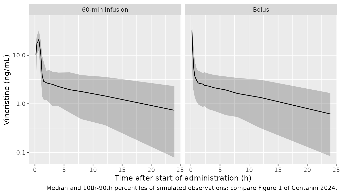
Infusion timing
TINF is the documented infusion duration, which the
model stretches by the estimated factor 1.30. The protocol infusion
lasted 60 min, of which 38 min were vincristine and 22 min flushing, so
the documented time could be either. The typical-value solve below (34
kg, 1.8 mg) compares the two readings with the observed median of Figure
1 (60-minute IV panel, read by the maintainers): about 24 ng/mL from
0.25 to 0.8 h, about 9 ng/mL at 1.1 h and about 3 ng/mL at 2.2 h.
tt <- c(0.25, 0.55, 0.85, 1.13, 2.2)
timing_events <- dplyr::bind_rows(
  tibble::tibble(id = 1:2, TINF = c(38 / 60, 1), time = 0, evid = 1L,
                 amt = 1.8, rate = -2),
  tidyr::expand_grid(tibble::tibble(id = 1:2, TINF = c(38 / 60, 1)),
                     time = tt) |>
    dplyr::mutate(evid = 0L, amt = 0, rate = 0)
) |>
  dplyr::mutate(cmt = "central", WT = 34, CYCLE = 1, PREV_AE_SCORE = 0) |>
  dplyr::arrange(id, time, dplyr::desc(evid))
timing <- rxode2::rxSolve(mod_typ, events = timing_events,
                          returnType = "data.frame") |>
  dplyr::select(id, time, Cc) |>
  tidyr::pivot_wider(names_from = id, values_from = Cc) |>
  dplyr::mutate(fig1 = c(24, 24, 19, 9, 3))
#> ℹ omega/sigma items treated as zero: 'etalcl', 'etalvc', 'etaltlag', 'etaRUV'
#> Warning: multi-subject simulation without without 'omega'
timing |>
  dplyr::rename("Time (h)" = time, "TINF = 38 min" = `1`,
                "TINF = 60 min" = `2`, "Figure 1 median (approx.)" = fig1) |>
  knitr::kable(digits = c(2, 1, 1, 0), caption = paste(
    "Typical concentrations (ng/mL) after a 1.8 mg infusion under the two",
    "readings of the documented infusion time."
))| Time (h) | TINF = 38 min | TINF = 60 min | Figure 1 median (approx.) |
|---|---|---|---|
| 0.25 | 18.9 | 11.9 | 24 |
| 0.55 | 24.2 | 15.3 | 24 |
| 0.85 | 25.7 | 16.3 | 19 |
| 1.13 | 6.0 | 17.0 | 9 |
| 2.20 | 2.9 | 3.0 | 3 |
With the 38-min drug time the infusion ends at about 0.9 h (38 min x
1.30 plus the 3.5-min lag) and the profile follows Figure 1; with 60 min
it would last 78 min, longer than the whole administration including the
flush, and the decline would come half an hour late. The vignette
therefore enters the standard infusion as TINF = 38/60
h.
PKNCA validation
The paper reports no NCA table. The check below runs PKNCA on the
simulated individual profiles (without residual error) and compares
AUC0-inf with the model’s own dose / CL, and the
body-surface-area-normalised clearance with the approximately 23 L/h/m^2
that the Discussion derives from the estimated CL.
sim_nca <- sim_pk |>
  dplyr::filter(!is.na(Cc)) |>
  dplyr::select(id, time, Cc, arm)
sim_nca <- dplyr::bind_rows(
  sim_nca,
  sim_nca |> dplyr::distinct(id, arm) |> dplyr::mutate(time = 0, Cc = 0)
) |>
  dplyr::distinct(id, arm, time, .keep_all = TRUE) |>
  dplyr::arrange(id, arm, time)

conc_obj <- PKNCA::PKNCAconc(sim_nca, Cc ~ time | arm + id)
dose_df <- pk_events |>
  dplyr::filter(evid == 1) |>
  dplyr::mutate(dose_ng = amt * 1e6) |>
  dplyr::select(id, time, dose_ng, arm)
dose_obj <- PKNCA::PKNCAdose(dose_df, dose_ng ~ time | arm + id)
intervals <- data.frame(
  start = 0, end = Inf,
  cmax = TRUE, tmax = TRUE, aucinf.obs = TRUE, half.life = TRUE
)
nca_res <- PKNCA::pk.nca(PKNCA::PKNCAdata(conc_obj, dose_obj,
                                          intervals = intervals))

nca_wide <- as.data.frame(nca_res) |>
  dplyr::filter(PPTESTCD %in% c("cmax", "tmax", "aucinf.obs", "half.life")) |>
  dplyr::select(id, arm, PPTESTCD, PPORRES) |>
  tidyr::pivot_wider(names_from = PPTESTCD, values_from = PPORRES)

auc_check <- nca_wide |>
  dplyr::inner_join(
    sim_pk |> dplyr::filter(time == 24) |>
      dplyr::select(id, auc_occ, cl, BSA),
    by = "id"
  ) |>
  dplyr::mutate(pct_diff = 100 * (aucinf.obs / auc_occ - 1),
                cl_bsa = cl / BSA)
stopifnot(
  # A fast-clearing subject can fall below solver precision before 72 h and
  # lose its terminal phase; nearly all subjects must still give AUC0-inf
  mean(is.na(auc_check$pct_diff)) < 0.05,
  # AUC0-inf from the simulated profile against dose / CL of the same
  # subject: numerical (trapezoid and extrapolation) error only
  abs(median(auc_check$pct_diff, na.rm = TRUE)) < 5,
  quantile(abs(auc_check$pct_diff), 0.9, na.rm = TRUE) < 15
)

nca_wide |>
  dplyr::group_by(arm) |>
  dplyr::summarise(
    cmax = median(cmax), tmax = median(tmax),
    aucinf = median(aucinf.obs, na.rm = TRUE),
    thalf = median(half.life, na.rm = TRUE),
    .groups = "drop"
  ) |>
  dplyr::rename(
    "Arm" = arm, "Cmax (ng/mL)" = cmax, "Tmax (h)" = tmax,
    "AUC0-inf (ng*h/mL)" = aucinf, "t1/2 (h)" = thalf
  ) |>
  knitr::kable(digits = 2,
caption = "Median simulated NCA parameters by arm (PKNCA).")| Arm | Cmax (ng/mL) | Tmax (h) | AUC0-inf (ng*h/mL) | t1/2 (h) |
|---|---|---|---|---|
| 60-min infusion | 21.98 | 0.67 | 64.73 | 10.79 |
| Bolus | 131.72 | 0.00 | 60.73 | 10.47 |
tibble::tibble(
  Quantity = "CL / BSA (L/h/m^2)",
  Simulated = median(auc_check$cl_bsa),
  Published = 23
) |>
  knitr::kable(digits = 1, caption = paste(
    "Median simulated BSA-normalised clearance against the Discussion's",
    "approximation of the estimated CL (Centanni 2024)."
))| Quantity | Simulated | Published |
|---|---|---|
| CL / BSA (L/h/m^2) | 23.2 | 23 |
The typical CL scaled to the cohort’s median weight and BSA gives 45.2 x (34/70)^0.75 / 1.2 = 21.8 L/h/m^2, close to the paper’s 23 L/h/m^2; the simulated median also reflects the weight and BSA spread of the virtual cohort.
Precision-dosing simulation, standard dosing arm (Table 4)
The paper simulated 1000 children with ALL receiving 1.5 mg/m^2 (cap
2 mg) over five occasions, with true exposures from the
_mipd model (mixture, IIV and IOV on CL), and reduced the
next dose by 20% after any grade >= 2 VIPN. The standard-dosing (“No
MIPD”) column of Table 4 gives the incidence of grade >= 2 VIPN (any
subscore) per occasion. The model-informed arm needs a Bayesian
dose-adaptation loop and is not reproduced here.
Each occasion below is one deterministic solve of the
_mipd model (random effects drawn in base R and passed as
parameters, so the cohort is machine-independent) that returns the VIPN
probabilities for a previous grade of 0 and above 0; the four subscore
chains are then sampled in R.
set.seed(20240202)
mod_mipd <- readModelDb("Centanni_2024_vincristine_mipd")
mod_mipd_typ <- rxode2::zeroRe(rxode2::rxode(mod_mipd))
#> ℹ parameter labels from comments will be replaced by 'label()'
#> Warning: some etas defaulted to non-mu referenced, possible parsing error: etalcl_oc1, etalcl_oc2, etalcl_oc3, etalcl_oc4, etalcl_oc5, etaRUV
#> as a work-around try putting the mu-referenced expression on a simple line
#> Warning: No sigma parameters in the model
#> Warning: some etas defaulted to non-mu referenced, possible parsing error: etalcl_oc1, etalcl_oc2, etalcl_oc3, etalcl_oc4, etalcl_oc5, etaRUV
#> as a work-around try putting the mu-referenced expression on a simple line
n_all <- 200
age_w <- c(3, 6, 6, 5, 4, 3.5, 3, 2.5, 2.2, 2, 2, 2, 2, 2, 2, 2, 2)
wt_anchor <- tibble::tibble(age = c(1, 2, 8.3, 18), wt = c(8.9, 11.5, 27.1, 70))
all_subjects <- tibble::tibble(
  id = seq_len(n_all),
  AGE = sample(1:17, n_all, replace = TRUE, prob = age_w) + runif(n_all),
  CYP3A5_EXPR = as.integer(runif(n_all) < 0.10),
  etalcl = rnorm(n_all, 0, sqrt(0.0992))
) |>
  dplyr::mutate(
    WT = exp(approx(log(wt_anchor$age), log(wt_anchor$wt), log(AGE),
                    rule = 2)$y) * exp(rnorm(n_all, 0, 0.15)),
    BSA = (4 * WT + 7) / (WT + 90),
    dose = pmin(1.5 * BSA, 2)
  )
iov <- matrix(rnorm(n_all * 5, 0, sqrt(0.1238)), n_all, 5)

subscores <- c("neuralgia", "motor", "constipation", "sensory")
grade_prev <- matrix(0, n_all, 4, dimnames = list(NULL, subscores))
dose_now <- all_subjects$dose
tox_prev <- rep(FALSE, n_all)
inc <- numeric(5)
exp_occ1 <- NA_real_
for (occ in 1:5) {
  dose_now <- ifelse(tox_prev, dose_now * 0.8, dose_now)
  ev <- dplyr::bind_rows(
    all_subjects |> dplyr::mutate(time = 0, evid = 1L, amt = dose_now,
                                  PREV_AE_SCORE = 0),
    all_subjects |> dplyr::mutate(time = 1, evid = 0L, amt = 0,
                                  PREV_AE_SCORE = 0),
    all_subjects |> dplyr::mutate(time = 2, evid = 0L, amt = 0,
                                  PREV_AE_SCORE = 1)
  ) |>
    dplyr::mutate(cmt = "central", TINF = 0, CYCLE = occ, OCC = occ) |>
    dplyr::arrange(id, time)
  prm <- all_subjects |>
    dplyr::select(id, etalcl) |>
    dplyr::mutate(etalcl_oc1 = iov[, 1], etalcl_oc2 = iov[, 2],
                  etalcl_oc3 = iov[, 3], etalcl_oc4 = iov[, 4],
                  etalcl_oc5 = iov[, 5])
  out <- rxode2::rxSolve(mod_mipd_typ, events = ev, params = prm,
                         returnType = "data.frame")
  p0 <- out[out$time == 1, ]
  p1 <- out[out$time == 2, ]
  tox <- rep(FALSE, n_all)
  p_none_ge2 <- rep(1, n_all)
  for (k in seq_along(subscores)) {
    prev_pos <- grade_prev[, k] > 0
    p_ge1 <- ifelse(prev_pos, p1$p_vipn_ge1, p0$p_vipn_ge1)
    p_ge2 <- if (subscores[k] %in% c("neuralgia", "motor")) {
      ifelse(prev_pos, p1$p_vipn_ge2_nm, p0$p_vipn_ge2_nm)
    } else {
      ifelse(prev_pos, p1$p_vipn_ge2_cs, p0$p_vipn_ge2_cs)
    }
    u <- runif(n_all)
    grade_prev[, k] <- ifelse(u < p_ge2, 2, ifelse(u < p_ge1, 1, 0))
    tox <- tox | grade_prev[, k] == 2
    p_none_ge2 <- p_none_ge2 * (1 - p_ge2)
  }
  # Occasion 1: every chain starts at grade 0, so the expected incidence is
  # exact given the cohort
  if (occ == 1) exp_occ1 <- 100 * mean(1 - p_none_ge2)
  inc[occ] <- 100 * mean(tox)
  tox_prev <- tox
}
#> ℹ omega/sigma items treated as zero: 'etalvc', 'etaltlag', 'etaRUV'
#> Warning: multi-subject simulation without without 'omega'
#> ℹ omega/sigma items treated as zero: 'etalvc', 'etaltlag', 'etaRUV'
#> Warning: multi-subject simulation without without 'omega'
#> ℹ omega/sigma items treated as zero: 'etalvc', 'etaltlag', 'etaRUV'
#> Warning: multi-subject simulation without without 'omega'
#> ℹ omega/sigma items treated as zero: 'etalvc', 'etaltlag', 'etaRUV'
#> Warning: multi-subject simulation without without 'omega'
#> ℹ omega/sigma items treated as zero: 'etalvc', 'etaltlag', 'etaRUV'
#> Warning: multi-subject simulation without without 'omega'

table4 <- tibble::tibble(
  occasion = 1:5,
  simulated = inc,
  published = c(5.8, 31.3, 51.4, 60.6, 62.1)
)
table4 |>
  dplyr::rename("Occasion" = occasion,
                "Simulated grade >= 2 (%)" = simulated,
                "Table 4, no MIPD (%)" = published) |>
  knitr::kable(digits = 1, caption = paste(
    "Incidence of grade >= 2 VIPN per occasion under standard dosing",
    "(1.5 mg/m^2, cap 2 mg, 20% reduction after grade >= 2)."
))| Occasion | Simulated grade >= 2 (%) | Table 4, no MIPD (%) |
|---|---|---|
| 1 | 4.5 | 5.8 |
| 2 | 36.5 | 31.3 |
| 3 | 53.0 | 51.4 |
| 4 | 62.5 | 60.6 |
| 5 | 64.5 | 62.1 |
exp_occ1
#> [1] 6.035305
stopifnot(
  # Occasion 1 expectation: with the printed AUC50 of 1.62 it is below 1%
  abs(exp_occ1 - 5.8) < 3,
  # Later occasions: centre of the four differences, robust to sampling
  abs(median(table4$simulated[2:5] - table4$published[2:5])) < 12
)
The first-occasion incidence is reproduced. Later occasions run a few percentage points above Table 4; part of that is sampling noise at 200 subjects, part is the virtual ALL cohort, whose age and weight distribution only approximates the paper’s CDC-based sampling, and part is the sensitivity to the occasion > 1 intercept described next.
Target exposure (Figure 3)
Figure 3 shows the probability of grade 0, 1 and >= 2 VIPN (any subscore), averaged over five occasions, against a fixed AUC per occasion. With no random effects in the VIPN model the subscore chains are independent Markov chains, so the probabilities follow exactly from the model outputs by propagating each chain’s grade distribution.
f3_grid <- c(0, 2.5, 5, seq(10, 120, by = 10))
f3_events <- tidyr::expand_grid(scen, auc = f3_grid) |>
  dplyr::mutate(id = dplyr::row_number())
f3_events <- dplyr::bind_rows(
  f3_events |> dplyr::mutate(time = 0, evid = 1L, amt = auc * 45.2 / 1000),
  f3_events |> dplyr::mutate(time = 24, evid = 0L, amt = 0)
) |>
  dplyr::mutate(cmt = "central", WT = 70, TINF = 0) |>
  dplyr::arrange(id, time)

propagate <- function(params = NULL) {
  pr <- rxode2::rxSolve(mod_typ, events = f3_events, params = params,
                        keep = c("auc"), returnType = "data.frame")
  pr$first <- pr$CYCLE == 1
  pr$prev <- pr$PREV_AE_SCORE > 0
  res <- lapply(f3_grid, function(a) {
    pa <- pr[pr$auc == a, ]
    # state distribution (grade 0, 1, >= 2) per subscore group
    dist <- list(nm = c(1, 0, 0), cs = c(1, 0, 0))
    ge1 <- ge2 <- numeric(5)
    for (occ in 1:5) {
      p_none_ge2 <- 1
      p_none_ge1 <- 1
      for (grp in c("nm", "cs")) {
        row0 <- pa[pa$first == (occ == 1) & !pa$prev, ]
        row1 <- pa[pa$first == (occ == 1) & pa$prev, ]
        col2 <- if (grp == "nm") "p_vipn_ge2_nm" else "p_vipn_ge2_cs"
        trans <- function(r) c(1 - r$p_vipn_ge1, r$p_vipn_ge1 - r[[col2]], r[[col2]])
        d <- dist[[grp]]
        new <- d[1] * trans(row0) + (d[2] + d[3]) * trans(row1)
        dist[[grp]] <- new
        # two subscores per group, independent chains
        p_none_ge2 <- p_none_ge2 * (1 - new[3])^2
        p_none_ge1 <- p_none_ge1 * new[1]^2
      }
      ge2[occ] <- 1 - p_none_ge2
      ge1[occ] <- 1 - p_none_ge1
    }
    tibble::tibble(auc = a, ge1 = mean(ge1), ge2 = mean(ge2))
  })
  dplyr::bind_rows(res)
}
f3 <- propagate()
#> ℹ omega/sigma items treated as zero: 'etalcl', 'etalvc', 'etaltlag', 'etaRUV'
#> Warning: multi-subject simulation without without 'omega'
f3_print <- propagate(c(b1_occ_vipn = -120, auc50_vipn = 0.164))
#> ℹ omega/sigma items treated as zero: 'etalcl', 'etalvc', 'etaltlag', 'etaRUV'
#> Warning: multi-subject simulation without without 'omega'

dplyr::bind_rows(
  f3 |> dplyr::mutate(model = "Packaged (B1|0, OCC > 1 = -119.54)"),
  f3_print |> dplyr::mutate(model = "B1|0, OCC > 1 = -120 (printed)")
) |>
  tidyr::pivot_longer(c(ge1, ge2), names_to = "grade", values_to = "p") |>
  dplyr::mutate(grade = ifelse(grade == "ge1", "Grade >= 1", "Grade >= 2")) |>
  ggplot(aes(auc, p, colour = grade, linetype = model)) +
  geom_line() +
  geom_hline(yintercept = 0.4, linetype = "dashed") +
  labs(x = "AUC per occasion (ng*h/mL)",
       y = "P(VIPN), mean of 5 occasions",
       colour = NULL, linetype = NULL,
       caption = paste0("Replicates Figure 3 of Centanni 2024 as cumulative\n",
                        "probabilities of grade >= 1 and grade >= 2.")) +
  theme(legend.position = "bottom", legend.direction = "vertical")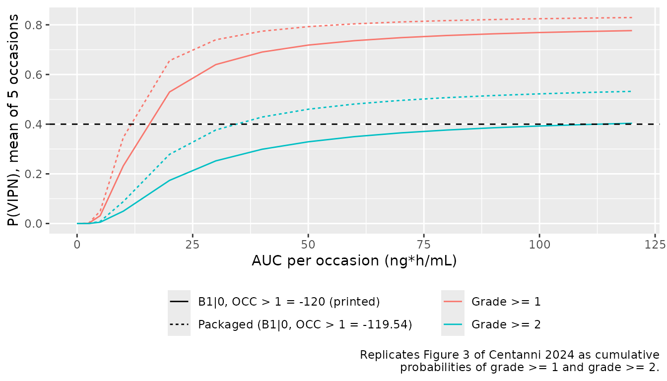
f3 |> dplyr::filter(auc %in% c(10, 20, 50, 100, 120)) |>
  dplyr::left_join(
    f3_print |> dplyr::select(auc, ge2_printed = ge2), by = "auc"
  ) |>
  dplyr::rename("AUC (ng*h/mL)" = auc, "Grade >= 1" = ge1,
                "Grade >= 2" = ge2, "Grade >= 2, intercept -120" = ge2_printed) |>
  knitr::kable(digits = 2, caption = paste(
    "Mean probability over five occasions. Figure 3 reads about 0.18, 0.37",
    "and 0.45 for grade >= 2 at 20, 50 and 100 ng*h/mL."
))| AUC (ng*h/mL) | Grade >= 1 | Grade >= 2 | Grade >= 2, intercept -120 |
|---|---|---|---|
| 10 | 0.35 | 0.09 | 0.05 |
| 20 | 0.66 | 0.28 | 0.17 |
| 50 | 0.79 | 0.46 | 0.33 |
| 100 | 0.82 | 0.52 | 0.39 |
| 120 | 0.83 | 0.53 | 0.40 |
Figure 3 lies between the two curves: about 0.18, 0.37 and 0.45 for grade >= 2 at 20, 50 and 100 ng*h/mL, against 0.28, 0.46 and 0.52 for the packaged model and 0.17, 0.33 and 0.39 with the occasion > 1 intercept at its printed -120. Figure S6 pins that intercept at -119.54 (its OCC1 curves sit 1.46 logit units above the first-occasion curves at every AUC), so the packaged model keeps the Figure S6 value. Figure 3 was simulated from 1000 virtual patients, and averaging over their exposure spread flattens the curve; the paper’s 50 ng*h/mL target corresponds to about 0.46 in the packaged model.
Assumptions and deviations
- AUC50. Table 3 prints 1.62 ng*h/mL. The packaged 0.164 ng*h/mL was fitted by the maintainers to the curves of Online Resource 2 (Figure S6), which the authors computed from the parameter estimates; the same fit recovers Emax, the Markov term, the grade >= 2 increment and the net first-occasion intercept of Table 3. With 1.62 the model predicts 0.6% grade >= 2 VIPN at the first occasion against the 5.8% of Table 4. No correction notice was found for the article (Europe PMC, 2026-10-29).
-
Occasion > 1 intercept. Table 3 prints -120. The
packaged -119.54 is the Figure S6 fit and rounds to the printed value;
b1_vipn = -121andemax_vipn = 119are as printed. Because the intercepts and Emax nearly cancel, use the packaged values together. - Subscore groups. Table 3 groups ‘neuropathy/motor’ against ‘constipation/sensory’. With sensory neuropathy in the second group, the first is read as neuralgia plus motor neuropathy, which is also how the 2026 follow-up code groups them.
-
Residual error. Table 2 reports the residual
magnitudes as ‘RUVadd’ on log-transformed data with IIV on the infusion
residual. IIV on a residual magnitude is coded in NONMEM as a theta
times
exp(eta)with the epsilon variance fixed to 1, so 0.137 and 0.204 are read as standard deviations on the log scale (lnorm). -
Infusion duration.
TINFis the documented infusion duration and the model infuses over1.30 x TINFafter the lag time. The paper does not say whether the documented time of the 60-min infusion is the 38 min of vincristine or the full 60 min with the flush; the maintainers read it as the 38-min drug time, which matches the timing of Figure 1 (see ‘Infusion timing’). Infusion dose records must carryrate = -2. -
Mixture on CL. The
_mipdmodel carries the paper’s latent two-group mixture as theCYP3A5_EXPRcovariate (1 = high-clearance group); the paper fixed the group probability to 10% rather than genotyping, so population simulations should draw it as Bernoulli(0.10). -
Occasion-level PK in the estimation model. In
Centanni_2024_vincristinethe IIV on CL is drawn once per subject. Since the paper treated each dosing occasion as its own individual, give each occasion its ownidto reproduce that structure, or use the_mipdmodel, which has explicit IOV. - Virtual cohorts. The weight distributions, the Costeff BSA (the paper used DuBois with sampled heights), the ALL age weights and the weight-for-age anchors are assumptions of this article. The paper sampled ages from published ALL incidence and weight and height from CDC LMS tables with a weight-height correlation of 0.7.
- Not reproduced. The model-informed dosing arm of Table 4 and Figures 4-5 (Bayesian estimation from three samples per occasion at 0.33, 6.5 and 7.5 h, a 50 ng*h/mL target with a 20% acceptance band) and the AUC accuracy comparison of MIPD against NCA.
- Population table. The text gives 20 bolus and 15 infusion patients; Table 1 labels the 20 (57%) row ‘Patients with infusion’.