Tafenoquine (Thakkar 2018)

Model and source

• Citation: Thakkar N, Green JA, Koh GCKW, Duparc S, Tenero D, Goyal N (2018). Population pharmacokinetics of tafenoquine, a novel antimalarial. Antimicrob Agents Chemother 62(11):e00711-18. doi:10.1128/AAC.00711-18.
• Description: Two-compartment first-order-absorption population PK model with an absorption lag time for oral tafenoquine, pooled across five phase 1 to phase 3 studies in healthy volunteers and Plasmodium vivax malaria patients (Thakkar 2018). Allometric body-weight scaling on CL/F, V2/F, Q/F and V3/F; capsule-versus-tablet formulation effects on relative bioavailability and on the absorption rate constant; and health status (healthy volunteer versus patient) on both apparent volumes of distribution. Interindividual variability is carried on CL/F and V2/F as a correlated block, plus Ka, the lag time, and the residual error magnitude.
• Article: https://doi.org/10.1128/AAC.00711-18
• Supplement (Tables S1-S3, Figures S1-S2): https://doi.org/10.1128/AAC.00711-18

Tafenoquine is an 8-aminoquinoline approved for the radical cure of acute Plasmodium vivax malaria, the first new treatment for that indication in almost 60 years. It is given as a single oral dose alongside standard chloroquine and has a long terminal half-life of roughly 15 days.

Population

The parameter-estimation data set pooled 5,286 plasma tafenoquine observations from 675 subjects across five studies spanning phase 1 to phase 3 (Thakkar 2018 Table 1): two healthy-volunteer tablet studies (200951, the drug-drug interaction study; 201780, the stable-isotope-label study), one healthy-volunteer capsule study (TAF114582, the thorough-QTc study), and the two parts of the TAF112582 DETECTIVE trial in P. vivax patients (part 1, phase 2B, capsule, dose-ranging over 50 to 600 mg; part 2, phase 3, tablet, 300 mg). Overall 193 subjects (28.6%) were healthy volunteers and 482 (71.4%) were patients; 297 (44.0%) received tablets and 378 (56.0%) capsules (Table 2). Median age was 35.0 years (range 15.0 to 79.0), median weight 69.3 kg (range 37.2 to 138), and 25.3% were female.

A sixth study, TAF116564 (GATHER, phase 3, 166 patients, tablet, 1,001 samples), was deliberately held out of estimation and used only for external validation. Its demographics are in Table S1 (median weight 64.8 kg, range 38.0 to 122.8; 31.3% female) and the paper states they “are highly comparable to the DETECTIVE part 2 (patient study) demographics”.

The same information is available programmatically via readModelDb("Thakkar_2018_tafenoquine")()$population.

Model structure

A two-compartment model with first-order absorption, a first-order absorption lag, and first-order elimination (Results, “Population PK model development”). Covariates enter through the paper’s two covariate forms:

• Equation 1 (continuous, power): P = theta_pop * (cov_ind / cov_med)^theta_cov. Body weight enters CL/F, V2/F, Q/F and V3/F allometrically with exponents fixed at 0.75 for the clearances and 1 for the volumes (Methods, “Covariate analysis”).
• Equation 2 (categorical, multiplicative): P = theta_pop * theta_cov^cat, so a subject in the reference cell (indicator 0) is unchanged. Formulation (FORM_CAPSULE, reference tablet) multiplies relative bioavailability by 0.863 and Ka by 0.924; health status (DIS_HEALTHY, reference P. vivax patient) multiplies V2/F by 1.35 and V3/F by 0.347.

Interindividual variability sits on CL/F and V2/F as a correlated block, plus Ka, the absorption lag, and the residual-error magnitude. IIV on Q/F and V3/F was tested and rejected by the authors, so neither carries an eta.

Source trace

Every ini() entry in inst/modeldb/specificDrugs/Thakkar_2018_tafenoquine.R carries an in-file comment naming its origin. They are collected here for review.

Equation / parameter	Value	Source location
lka	0.252 1/h	Table 3, “K a (h-1)”
lcl	2.96 L/h	Table 3, “CL/F (liters/h)”
lvc	915 L	Table 3, “V 2/F (liters)”
lq	5.09 L/h	Table 3, “Q/F (liters/h)”
lvp	664 L	Table 3, “V 3/F (liters)”
ltlag	0.908 h	Table 3, “Absorption lag time (h)”
lfdepot	1 (fixed)	Table 3 footnote a, “the tablet formulation was considered the reference, i.e., F 1tablet = 1”
e_wt_cl_q	0.75 (fixed)	Methods, “Covariate analysis”: “Fixed exponents of 0.75 and 1 were applied for the clearance and volume parameters”
e_wt_vc_vp	1 (fixed)	Methods, “Covariate analysis” (same sentence)
e_form_capsule_fdepot	0.863	Table 3, “Relative bioavailability (capsule)”
e_form_capsule_ka	0.924	Table 3, “Capsule effect on K a”
e_dis_healthy_vc	1.35	Table 3, “V 2/F ratio (healthy volunteers/patients)”
e_dis_healthy_vp	0.347	Table 3, “V 3/F ratio (healthy volunteers/patients)”
etalcl	0.09807	Table 3, “IIV CL/F” = 32.1% CV; log(1 + 0.321^2)
etalvc	0.11184	Table 3, “IIV V 2/F” = 34.4% CV; log(1 + 0.344^2)
cov(etalcl, etalvc)	0.03488	Table 3, “IIV CL-V 2 block” = 33.3 read as a correlation (see Assumptions)
etalka	0.15119	Table 3, “IIV K a” = 40.4% CV; log(1 + 0.404^2)
etaltlag	0.17919	Table 3, “IIV ALAG1” = 44.3% CV; log(1 + 0.443^2)
expSd	0.14917	Table 3, “Random residual variability (% CV)” = 15.0; sqrt(log(1 + 0.150^2))
etaexpSd	0.10337	Table 3, “IIV error” = 33.0% CV; log(1 + 0.330^2)
Structure: 2-compartment, first-order absorption + lag	n/a	Results, “Population PK model development”; Final model paragraph
Equation 1 (continuous power covariate)	n/a	Methods, “Covariate analysis”, equation 1
Equation 2 (categorical multiplicative covariate)	n/a	Methods, “Covariate analysis”, equation 2
Residual: additive on log-transformed data = exponential	n/a	Methods, “Population PK model development”

Deterministic structural checks

Before simulating a cohort, the typical-value predictions are checked against quantities that follow in closed form from the published parameters. These are deterministic (zeroRe()), so the tolerances below are numerical-integration tolerances, not sampling tolerances.

mod <- readModelDb("Thakkar_2018_tafenoquine")
mod_typ <- rxode2::zeroRe(mod)
#> ℹ parameter labels from comments will be replaced by 'label()'
#> Warning: No sigma parameters in the model

# Fine early sampling to resolve Tmax, then out to 180 days so that the
# terminal slope and the extrapolated AUC are well determined.
t_typ <- sort(unique(c(
  seq(0, 24, by = 0.1),
  seq(24, 72, by = 0.5),
  seq(72, 1440, by = 6),
  seq(1440, 180 * 24, by = 24)
)))

# One subject per covariate cell, all at the same weight so that the
# formulation and health-status contrasts are not confounded by allometry.
cells <- tibble::tibble(
  cell = c("Patient, tablet", "Patient, capsule", "Healthy, tablet", "Healthy, capsule"),
  FORM_CAPSULE = c(0, 1, 0, 1),
  DIS_HEALTHY = c(0, 0, 1, 1)
) |>
  dplyr::mutate(id = dplyr::row_number(), WT = 64.8)

ev_typ <- dplyr::bind_rows(
  cells |> dplyr::mutate(time = 0, amt = 300, evid = 1L, cmt = "depot"),
  cells |>
    tidyr::crossing(time = t_typ) |>
    dplyr::mutate(amt = NA_real_, evid = 0L, cmt = "central")
) |>
  dplyr::arrange(id, time, dplyr::desc(evid))

sim_typ <- rxode2::rxSolve(
  mod_typ,
  events = ev_typ,
  keep = c("cell", "WT", "FORM_CAPSULE", "DIS_HEALTHY")
) |>
  as.data.frame() |>
  dplyr::filter(!is.na(Cc))
#> ℹ omega/sigma items treated as zero: 'etalcl', 'etalvc', 'etalka', 'etaltlag', 'etaexpSd'
#> Warning: multi-subject simulation without without 'omega'

stopifnot(nrow(sim_typ) > 0, all(sim_typ$Cc >= 0))

# Trapezoidal helper used only for the closed-form comparisons below; the
# reported NCA in this vignette is computed by PKNCA further down.
trap <- function(x, y) sum(diff(x) * (utils::head(y, -1) + utils::tail(y, -1)) / 2)

typ_sum <- sim_typ |>
  dplyr::filter(time > 0) |>
  dplyr::group_by(cell, FORM_CAPSULE, DIS_HEALTHY, WT) |>
  dplyr::summarise(
    cmax = max(Cc),
    tmax = time[which.max(Cc)],
    auc_0_60d = trap(time[time <= 1440], Cc[time <= 1440]),
    auc_0_180d = trap(time, Cc),
    .groups = "drop"
  )

knitr::kable(
  typ_sum |>
    dplyr::select(cell, cmax, tmax, auc_0_60d, auc_0_180d) |>
    dplyr::rename(
      "Covariate cell" = cell,
      "Cmax (ng/mL)" = cmax,
      "Tmax (h)" = tmax,
      "AUC0-60d (ng*h/mL)" = auc_0_60d,
      "AUC0-180d (ng*h/mL)" = auc_0_180d
    ),
  digits = c(0, 1, 2, 0, 0),
  caption = "Typical-value predictions after a single 300 mg oral dose at 64.8 kg."
)

Typical-value predictions after a single 300 mg oral dose at 64.8 kg.

Covariate cell	Cmax (ng/mL)	Tmax (h)	AUC0-60d (ng*h/mL)	AUC0-180d (ng*h/mL)
Healthy, capsule	205.4	17.3	87710	92667
Healthy, tablet	239.2	16.3	101637	107378
Patient, capsule	269.0	15.7	85658	92632
Patient, tablet	313.9	14.8	99260	107338

# Closed-form typical values at WT = 64.8 kg.
wt_ref <- 64.8
cl_typ <- 2.96 * (wt_ref / 70)^0.75
q_typ <- 5.09 * (wt_ref / 70)^0.75
vc_pat <- 915 * (wt_ref / 70)
vp_pat <- 664 * (wt_ref / 70)

# Terminal rate constant is the smaller eigenvalue of the two-compartment
# disposition matrix.
beta_of <- function(cl, vc, q, vp) {
  k10 <- cl / vc
  k12 <- q / vc
  k21 <- q / vp
  s <- k10 + k12 + k21
  0.5 * (s - sqrt(s^2 - 4 * k21 * k10))
}
thalf_pat_d <- log(2) / beta_of(cl_typ, vc_pat, q_typ, vp_pat) / 24
thalf_hv_d <- log(2) / beta_of(cl_typ, vc_pat * 1.35, q_typ, vp_pat * 0.347) / 24

pick <- function(nm, col) typ_sum[[col]][typ_sum$cell == nm]

# 1. AUC to infinity is Dose * F / CL exactly. The 180-day integral is about
#    10 terminal half-lives, so it misses under 0.1% of the tail, and the
#    trapezoidal rule adds a comparably tiny overshoot on a convex decay.
#    Deterministic, so 2% is pure numerical tolerance; a wrong CL, a missing
#    bioavailability term or a wrong concentration unit breaks it by 10% or
#    much more.
auc_inf_closed <- 1000 * 300 / cl_typ
rel_auc <- pick("Patient, tablet", "auc_0_180d") / auc_inf_closed
stopifnot(abs(rel_auc - 1) < 0.02)

# 2. Relative bioavailability is the ONLY structural difference that moves AUC
#    between formulations (the Ka effect cannot change AUC), so the ratio must
#    reproduce 0.863 to integration accuracy.
ratio_form <- pick("Patient, capsule", "auc_0_180d") / pick("Patient, tablet", "auc_0_180d")
stopifnot(abs(ratio_form - 0.863) < 0.005)

# 3. Health status acts on the volumes ONLY. CL/F carries no health-status
#    term, so AUC must be unchanged between the two health strata. This gate
#    fails loudly if the covariate is ever mis-attached to clearance.
ratio_hv <- pick("Healthy, tablet", "auc_0_180d") / pick("Patient, tablet", "auc_0_180d")
stopifnot(abs(ratio_hv - 1) < 0.01)

# 4. Terminal half-life. Every micro-constant of this model scales as
#    (WT/70)^-0.25, so t1/2 scales as (WT/70)^0.25 and the closed-form values
#    below are weight-dependent: 16.9 days for a 64.8 kg patient and 17.2 days
#    at 70 kg. Both bracket the "approximately 15 days" quoted in the paper's
#    Introduction, which is the only published figure to check against, so the
#    window is anchored on that statement rather than on a value read off this
#    run. The tight comparison is against the SIMULATED half-life further
#    down, which uses this closed form as its reference.
stopifnot(
  thalf_pat_d > 14, thalf_pat_d < 20,
  thalf_hv_d > 12, thalf_hv_d < 18,
  thalf_hv_d < thalf_pat_d
)

# 5. Tmax is the Ka-sensitive quantity here; Cmax is NOT. With
#    ka / kel = 0.252 / (2.96/915) = 78, absorption is ~80-fold faster than
#    elimination, so Cmax sits close to Dose/V2 and barely moves with Ka. The
#    capsule's 0.924 factor on Ka must therefore show up as a LATER Tmax, not
#    as a lower Cmax beyond the bioavailability effect. Deterministic solve, so
#    the ordering below is exact rather than a sampling coin flip.
tmax_tab <- pick("Patient, tablet", "tmax")
tmax_cap <- pick("Patient, capsule", "tmax")
stopifnot(
  tmax_tab > 10, tmax_tab < 25,
  tmax_cap > tmax_tab
)

tibble::tibble(
  Check = c(
    "AUC0-180d / (Dose/CL), patient tablet",
    "AUC capsule / AUC tablet (expect 0.863)",
    "AUC healthy / AUC patient (expect 1; CL has no health term)",
    "Terminal t1/2, patient (days)",
    "Terminal t1/2, healthy volunteer (days)",
    "Tmax tablet (h)",
    "Tmax capsule (h)"
  ),
  Value = c(rel_auc, ratio_form, ratio_hv, thalf_pat_d, thalf_hv_d, tmax_tab, tmax_cap)
) |>
  knitr::kable(digits = 4, caption = "Deterministic structural checks (all gated with stopifnot above).")

Deterministic structural checks (all gated with stopifnot above).

Check	Value
AUC0-180d / (Dose/CL), patient tablet	0.9995
AUC capsule / AUC tablet (expect 0.863)	0.8630
AUC healthy / AUC patient (expect 1; CL has no health term)	1.0004
Terminal t1/2, patient (days)	16.8918
Terminal t1/2, healthy volunteer (days)	14.2455
Tmax tablet (h)	14.8000
Tmax capsule (h)	15.7000

# Typical-value profiles for the four covariate cells. This is the structural
# content of Figure S1 (health status on V2/F): at equal dose and weight the
# healthy volunteer has the higher central volume and therefore the LOWER
# early concentration, which is what the authors added the covariate to fix.
sim_typ |>
  dplyr::filter(time > 0, time <= 60 * 24) |>
  ggplot(aes(time / 24, Cc, colour = cell, linetype = cell)) +
  geom_line(linewidth = 0.7) +
  scale_y_log10() +
  labs(
    x = "Time (days)", y = "Tafenoquine (ng/mL)",
    colour = NULL, linetype = NULL,
    title = "Typical-value profiles by covariate cell, 300 mg single oral dose",
    caption = "Structural content of Figure S1 of Thakkar 2018; all cells at 64.8 kg."
  ) +
  theme(legend.position = "bottom")
#> Warning in scale_y_log10(): log-10 transformation introduced infinite values.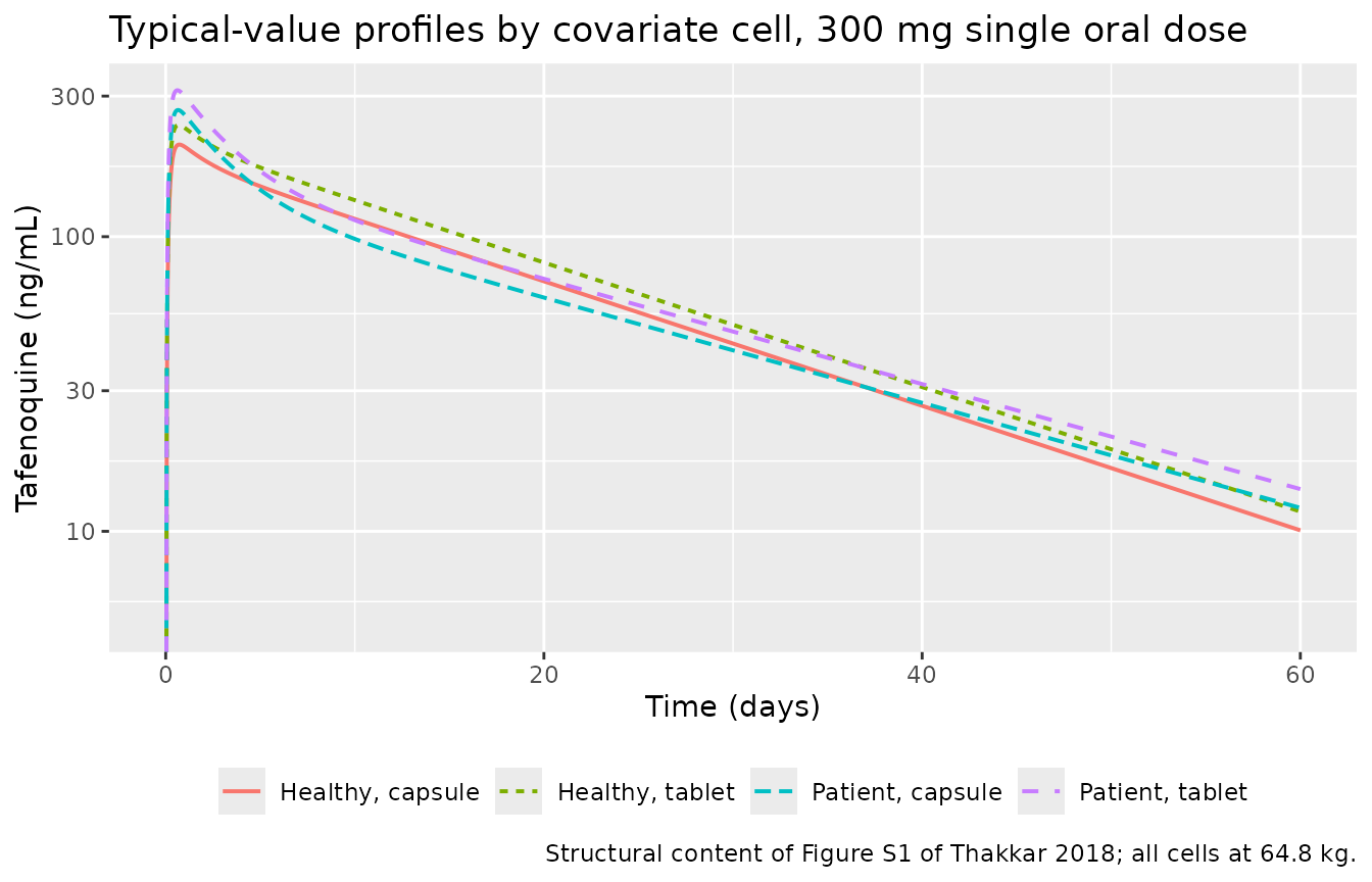

Virtual cohort

Original observed data are not publicly available, so the cohort below approximates the published per-study demographics. Weights are drawn from a log-normal truncated to the published range.

Patient-study weights use the GATHER median of 64.8 kg and range 38.0 to 122.8 kg (Table S1); the paper states GATHER demographics are “highly comparable to the DETECTIVE part 2 (patient study) demographics”, and DETECTIVE parts 1 and 2 are parts of one protocol (TAF112582), so the same distribution is used for all three patient arms. The healthy-volunteer arm uses the pooled analysis-set median of 69.3 kg and range 37.2 to 138 kg (Table 2), which is the only weight summary published for those studies.

# set.seed() seeds R's RNG. It does NOT seed rxode2's simulation RNG, and
# rxode2's streams are partitioned per solver thread, so the cohort below
# differs between a 2-core CI runner and a 16-thread workstation. Every
# assertion downstream is written to hold for any cohort the model can draw.
set.seed(20181128)

# 200 per arm is the per-arm cap. It is used rather than something smaller
# because the comparison against Table S2 below is a comparison of MEDIANS,
# and the Monte Carlo error of a median scales as 1/sqrt(n): at 130 per arm
# the two structurally identical tablet arms (DETECTIVE part 2 and GATHER)
# landed 4 percentage points apart on AUC purely by draw, at 200 they agree
# to under 0.2. That noise floor is what sets the gate tolerances below.
n_arm <- 200L

rtrunc_lnorm <- function(n, med, lo, hi, sdlog = 0.22) {
  meanlog <- log(med)
  u <- stats::runif(n, stats::plnorm(lo, meanlog, sdlog), stats::plnorm(hi, meanlog, sdlog))
  stats::qlnorm(u, meanlog, sdlog)
}

# Observation grid: dense enough early to resolve Cmax / Tmax, then daily out
# to exactly 1440 h (60 days) so AUC0-60 lines up with Table S2.
t_cohort <- sort(unique(c(
  seq(0, 12, by = 0.5),
  seq(13, 30, by = 1),
  seq(33, 72, by = 3),
  seq(96, 1440, by = 24)
)))
stopifnot(1440 %in% t_cohort)

make_arm <- function(n, study, form_capsule, dis_healthy, wt_med, wt_lo, wt_hi, id_offset) {
  subj <- tibble::tibble(
    id = id_offset + seq_len(n),
    study = study,
    FORM_CAPSULE = form_capsule,
    DIS_HEALTHY = dis_healthy,
    WT = rtrunc_lnorm(n, wt_med, wt_lo, wt_hi)
  )
  dplyr::bind_rows(
    subj |> dplyr::mutate(time = 0, amt = 300, evid = 1L, cmt = "depot"),
    subj |>
      tidyr::crossing(time = t_cohort) |>
      dplyr::mutate(amt = NA_real_, evid = 0L, cmt = "central")
  ) |>
    dplyr::arrange(id, time, dplyr::desc(evid))
}

events <- dplyr::bind_rows(
  make_arm(n_arm, "DETECTIVE part 1 (capsule)", 1, 0, 64.8, 38.0, 122.8, id_offset = 0L),
  make_arm(n_arm, "DETECTIVE part 2 (tablet)", 0, 0, 64.8, 38.0, 122.8, id_offset = 1000L),
  make_arm(n_arm, "GATHER (tablet)", 0, 0, 64.8, 38.0, 122.8, id_offset = 2000L),
  make_arm(n_arm, "TQT (capsule, healthy)", 1, 1, 69.3, 37.2, 138.0, id_offset = 3000L)
)

stopifnot(!anyDuplicated(unique(events[, c("id", "time", "evid")])))

Simulation

sim <- rxode2::rxSolve(
  mod,
  events = events,
  keep = c("study", "WT", "FORM_CAPSULE", "DIS_HEALTHY")
) |>
  as.data.frame()
#> ℹ parameter labels from comments will be replaced by 'label()'

stopifnot(nrow(sim) > 0, !all(is.na(sim$Cc)))

# Replicates the shape of Figure 2 of Thakkar 2018: median and 95% prediction
# interval of the simulated concentration-time profile by study, 300 mg.
sim |>
  dplyr::filter(!is.na(Cc), time > 0) |>
  dplyr::group_by(study, time) |>
  dplyr::summarise(
    Q025 = stats::quantile(Cc, 0.025),
    Q50 = stats::median(Cc),
    Q975 = stats::quantile(Cc, 0.975),
    .groups = "drop"
  ) |>
  ggplot(aes(time / 24, Q50)) +
  geom_ribbon(aes(ymin = Q025, ymax = Q975), alpha = 0.25, fill = "steelblue") +
  geom_line(colour = "steelblue4", linewidth = 0.7) +
  facet_wrap(~study) +
  scale_y_log10() +
  labs(
    x = "Time (days)", y = "Tafenoquine (ng/mL)",
    title = "Simulated median and 95% prediction interval, 300 mg single oral dose",
    caption = "Replicates Figure 2 of Thakkar 2018 (and Figure S2 for the TQT study)."
  )
#> Warning in scale_y_log10(): log-10 transformation introduced infinite values.
#> log-10 transformation introduced infinite values.
#> log-10 transformation introduced infinite values.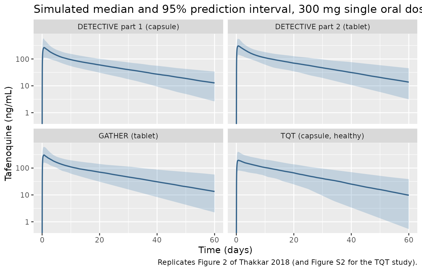

PKNCA validation

sim_nca <- sim |>
  dplyr::filter(!is.na(Cc)) |>
  dplyr::select(id, time, Cc, study)

# Guarantee a time = 0 row per subject; pre-dose Cc = 0 is correct for an
# extravascular single dose.
sim_nca <- dplyr::bind_rows(
  sim_nca,
  sim_nca |> dplyr::distinct(id, study) |> dplyr::mutate(time = 0, Cc = 0)
) |>
  dplyr::distinct(id, study, time, .keep_all = TRUE) |>
  dplyr::arrange(id, study, time)

stopifnot(all(sim_nca$Cc >= 0))

conc_obj <- PKNCA::PKNCAconc(sim_nca, Cc ~ time | study + id)

dose_df <- events |>
  dplyr::filter(evid == 1L) |>
  dplyr::select(id, time, amt, study)
dose_obj <- PKNCA::PKNCAdose(dose_df, amt ~ time | study + id)

# AUC0-60 in Table S2 is the AUC to day 60, so the interval ends at 1440 h,
# which is also the last sampled time. One interval row with every requested
# parameter: bind_rows()-ing two partially-specified rows would leave NA in
# the unshared logical columns and PKNCA rejects that.
intervals <- data.frame(
  start = 0, end = 1440,
  auclast = TRUE, cmax = TRUE, tmax = TRUE, half.life = TRUE
)

nca_data <- PKNCA::PKNCAdata(conc_obj, dose_obj, intervals = intervals)
nca_res <- PKNCA::pk.nca(nca_data)

Comparison against published predicted exposures

Thakkar 2018 Table S2 reports the median and 5th-95th percentile of AUC0-60 and Cmax at the 300 mg dose, predicted from 500 bootstrap model runs over each study’s own subject demographics. Those medians are the reference values below. AUC is converted from ugh/mL to ngh/mL to match the model’s ng/mL concentration unit.

published <- tibble::tribble(
  ~study,                        ~auclast,  ~cmax,
  "DETECTIVE part 1 (capsule)",  93.19e3,   296.98,
  "DETECTIVE part 2 (tablet)",  101.66e3,   322.42,
  "GATHER (tablet)",            100.14e3,   315.45
)

cmp <- nlmixr2lib::ncaComparisonTable(
  simulated = nca_res,
  reference = published,
  by = "study",
  params = c("cmax", "auclast"),
  units = c(cmax = "ng/mL", auclast = "ng*h/mL"),
  tolerance_pct = 20
)

knitr::kable(
  cmp,
  digits = 1,
  caption = "Simulated vs Thakkar 2018 Table S2 predicted exposures at 300 mg. * differs by >20%."
)

Simulated vs Thakkar 2018 Table S2 predicted exposures at 300 mg. * differs by >20%.

NCA parameter	study	Reference	Simulated	% diff
Cmax (ng/mL)	DETECTIVE part 1 (capsule)	297	266	-10.4%
Cmax (ng/mL)	DETECTIVE part 2 (tablet)	322	314	-2.6%
Cmax (ng/mL)	GATHER (tablet)	315	311	-1.6%
AUClast (ng*h/mL)	DETECTIVE part 1 (capsule)	93200	82500	-11.5%
AUClast (ng*h/mL)	DETECTIVE part 2 (tablet)	102000	99100	-2.5%
AUClast (ng*h/mL)	GATHER (tablet)	100000	97500	-2.6%

attr(cmp, "footnote")
#> NULL

# `cmp`'s "% diff" column is a formatted character string, so the gate is
# recomputed numerically from the same medians ncaComparisonTable() uses.
sim_med <- as.data.frame(nca_res) |>
  dplyr::filter(PPTESTCD %in% c("cmax", "auclast")) |>
  dplyr::group_by(study, PPTESTCD) |>
  dplyr::summarise(median = stats::median(PPORRES, na.rm = TRUE), .groups = "drop") |>
  tidyr::pivot_wider(names_from = PPTESTCD, values_from = median)

pct <- published |>
  dplyr::inner_join(sim_med, by = "study", suffix = c("_ref", "_sim")) |>
  dplyr::mutate(
    pct_cmax = 100 * (cmax_sim / cmax_ref - 1),
    pct_auc = 100 * (auclast_sim / auclast_ref - 1)
  )
stopifnot(nrow(pct) == 3L)

# Realised deviations at 200/arm: Cmax -10.4 / -2.6 / -1.6 %, AUC -11.5 /
# -2.5 / -2.6 % for DETECTIVE part 1 / part 2 / GATHER. The worst arm is the
# capsule one, where the unpublished DETECTIVE part 1 weight distribution is
# the dominant unknown; the residual per-arm Monte Carlo error on a
# 200-subject median is about 3 points. The gate therefore sits at 25, which
# clears the realised worst case by roughly four standard errors while still
# going red on a mis-transcribed clearance, dose or concentration unit -- any
# of which move exposure by tens of percent or more.
stopifnot(max(abs(c(pct$pct_cmax, pct$pct_auc))) < 25)

Simulated NCA by study

nca_wide <- as.data.frame(nca_res) |>
  dplyr::filter(PPTESTCD %in% c("cmax", "tmax", "auclast", "half.life")) |>
  dplyr::group_by(study, PPTESTCD) |>
  dplyr::summarise(
    median = stats::median(PPORRES, na.rm = TRUE),
    p05 = stats::quantile(PPORRES, 0.05, na.rm = TRUE),
    p95 = stats::quantile(PPORRES, 0.95, na.rm = TRUE),
    .groups = "drop"
  )

nca_wide |>
  dplyr::mutate(
    PPTESTCD = dplyr::recode(
      PPTESTCD,
      cmax = "Cmax (ng/mL)", tmax = "Tmax (h)",
      auclast = "AUC0-60 (ng*h/mL)", half.life = "t1/2 (h)"
    )
  ) |>
  dplyr::rename(
    "Study" = study, "NCA parameter" = PPTESTCD,
    "Median" = median, "5th pctile" = p05, "95th pctile" = p95
  ) |>
  knitr::kable(digits = 1, caption = "Simulated NCA summary by study, 300 mg single oral dose.")

Simulated NCA summary by study, 300 mg single oral dose.

Study	NCA parameter	Median	5th pctile	95th pctile
DETECTIVE part 1 (capsule)	AUC0-60 (ng*h/mL)	82490.6	54727.2	133838.4
DETECTIVE part 1 (capsule)	Cmax (ng/mL)	266.1	132.1	506.4
DETECTIVE part 1 (capsule)	t1/2 (h)	412.9	269.4	703.2
DETECTIVE part 1 (capsule)	Tmax (h)	15.5	10.5	25.0
DETECTIVE part 2 (tablet)	AUC0-60 (ng*h/mL)	99090.9	61243.0	155827.9
DETECTIVE part 2 (tablet)	Cmax (ng/mL)	314.2	170.5	520.8
DETECTIVE part 2 (tablet)	t1/2 (h)	404.0	268.6	633.2
DETECTIVE part 2 (tablet)	Tmax (h)	16.0	10.0	25.0
GATHER (tablet)	AUC0-60 (ng*h/mL)	97493.1	57539.9	176723.2
GATHER (tablet)	Cmax (ng/mL)	310.5	166.1	572.8
GATHER (tablet)	t1/2 (h)	405.2	256.3	751.5
GATHER (tablet)	Tmax (h)	15.0	10.0	23.0
TQT (capsule, healthy)	AUC0-60 (ng*h/mL)	83868.3	42851.9	154600.1
TQT (capsule, healthy)	Cmax (ng/mL)	196.2	95.2	381.0
TQT (capsule, healthy)	t1/2 (h)	345.4	193.4	588.6
TQT (capsule, healthy)	Tmax (h)	18.0	11.5	29.0

# Median simulated terminal half-life across the patient arms should sit near
# the closed-form 17.2 days derived from the published CL/F, V2/F, Q/F and
# V3/F. Loose enough to tolerate a different cohort draw, tight enough that a
# mis-transcribed disposition parameter breaks it.
hl_pat <- nca_wide |>
  dplyr::filter(PPTESTCD == "half.life", study != "TQT (capsule, healthy)")
stopifnot(nrow(hl_pat) == 3)
stopifnot(all(abs(hl_pat$median / 24 / thalf_pat_d - 1) < 0.15))

Relative bioavailability across formulations

Thakkar 2018 Table 4 reports the point estimate and 90% CI of the tablet / capsule exposure ratio computed from post hoc individual estimates, and concludes that both ratios sit inside the 80-125% bioequivalence limits. The same contrast computed from this simulation is shown below. Note that the published ratios are between different study populations, so they also carry the between-study demographic difference; the model-only contrast at matched weight is the structural 1 / 0.863 = 1.159 checked deterministically above.

med_by_study <- nca_wide |>
  dplyr::filter(PPTESTCD %in% c("cmax", "auclast")) |>
  dplyr::select(study, PPTESTCD, median) |>
  tidyr::pivot_wider(names_from = PPTESTCD, values_from = median)

getm <- function(s, p) med_by_study[[p]][med_by_study$study == s]
cap <- "DETECTIVE part 1 (capsule)"

rel_tab <- tibble::tibble(
  Comparison = c(
    "DETECTIVE part 2 (tablet) vs DETECTIVE part 1 (capsule)",
    "GATHER (tablet) vs DETECTIVE part 1 (capsule)"
  ),
  `AUC ratio, simulated` = c(
    getm("DETECTIVE part 2 (tablet)", "auclast") / getm(cap, "auclast"),
    getm("GATHER (tablet)", "auclast") / getm(cap, "auclast")
  ),
  `AUC ratio, Table 4` = c(1.07, 1.00),
  `Cmax ratio, simulated` = c(
    getm("DETECTIVE part 2 (tablet)", "cmax") / getm(cap, "cmax"),
    getm("GATHER (tablet)", "cmax") / getm(cap, "cmax")
  ),
  `Cmax ratio, Table 4` = c(1.00, 0.90)
)

knitr::kable(rel_tab, digits = 3, caption = "Tablet / capsule exposure ratios: simulated vs Thakkar 2018 Table 4.")

Tablet / capsule exposure ratios: simulated vs Thakkar 2018 Table 4.

Comparison	AUC ratio, simulated	AUC ratio, Table 4	Cmax ratio, simulated	Cmax ratio, Table 4
DETECTIVE part 2 (tablet) vs DETECTIVE part 1 (capsule)	1.201	1.07	1.180	1.0
GATHER (tablet) vs DETECTIVE part 1 (capsule)	1.182	1.00	1.167	0.9

# These cross-arm ratios are each a quotient of two INDEPENDENT cohort
# medians, so they carry roughly 3 points of Monte Carlo error on top of the
# structural 1 / 0.863 = 1.159. Realised at 200/arm: AUC 1.201 and 1.182,
# Cmax 1.181 and 1.167. The window below clears both sides by about four
# standard errors and still goes red on the failure that matters -- dropping
# or mis-signing the relative-bioavailability term would put every ratio at
# about 1.0. The exact structural contrast is gated deterministically in the
# "Deterministic structural checks" section above; this is only a sanity
# bound on the cohort version of it.
stopifnot(
  all(rel_tab$`AUC ratio, simulated` > 1.05),
  all(rel_tab$`AUC ratio, simulated` < 1.35),
  all(rel_tab$`Cmax ratio, simulated` > 1.05),
  all(rel_tab$`Cmax ratio, simulated` < 1.35)
)

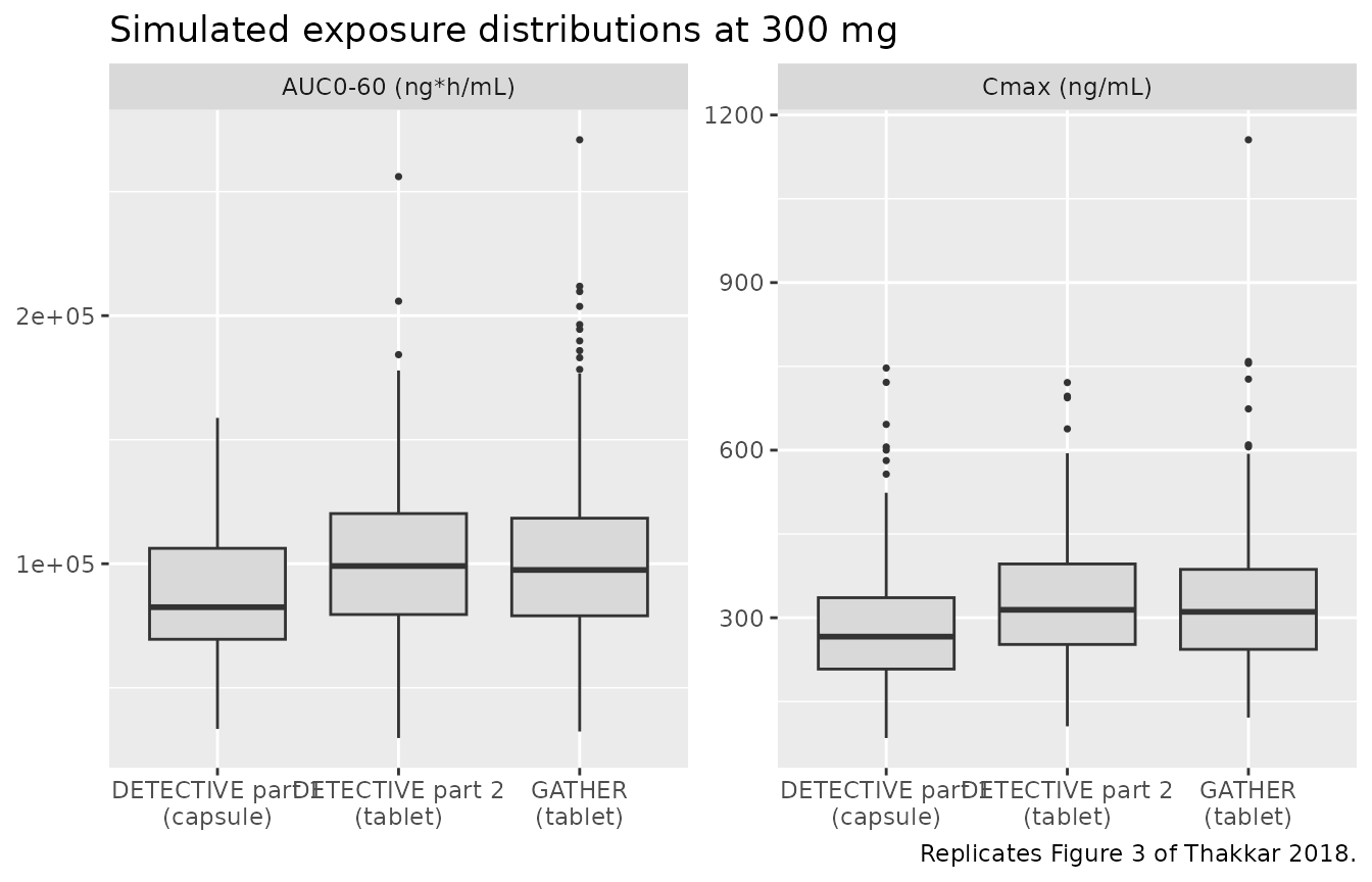
# Replicates Figure 3 of Thakkar 2018: distribution of post hoc AUC0-60 and
# Cmax at 300 mg across studies.
as.data.frame(nca_res) |>
  dplyr::filter(
    PPTESTCD %in% c("auclast", "cmax"),
    study != "TQT (capsule, healthy)"
  ) |>
  dplyr::mutate(
    PPTESTCD = dplyr::recode(
      PPTESTCD,
      auclast = "AUC0-60 (ng*h/mL)", cmax = "Cmax (ng/mL)"
    )
  ) |>
  ggplot(aes(study, PPORRES)) +
  geom_boxplot(fill = "grey85", outlier.size = 0.6) +
  facet_wrap(~PPTESTCD, scales = "free_y") +
  scale_x_discrete(labels = function(x) sub(" \\(", "\n(", x)) +
  labs(
    x = NULL, y = NULL,
    title = "Simulated exposure distributions at 300 mg",
    caption = "Replicates Figure 3 of Thakkar 2018."
  )

Assumptions and deviations

• Allometric reference weight. The paper applies allometric scaling with exponents fixed at 0.75 and 1 but never states the normalising weight; the conventional 70 kg is used. The analysis-set median is 69.3 kg (Table 2), so the choice shifts typical clearances by (69.3/70)^0.75 = 0.993 and typical volumes by 69.3/70 = 0.990 relative to normalising at the median instead. Either choice is absorbed into the reported typical values and neither changes any ratio checked in this vignette.

• The OMEGA block off-diagonal is read as a correlation, not a %CV. Table 3 footnote a says the IIV rows are “expressed as the percent coefficient of variation”, and the row “IIV CL-V 2 block” reports 33.3. Applying the %CV transform used for the diagonals gives an off-diagonal of log(1 + 0.333^2) = 0.10516, which divided by sqrt(0.09807 * 0.11184) = 0.10473 implies a correlation of 1.004 – outside [-1, 1], so that reading is arithmetically impossible and the matrix would not be positive definite. Reading 33.3 as a correlation of 0.333 (the usual NONMEM / PsN convention for a $OMEGA BLOCK off-diagonal reported alongside %CV diagonals) gives a covariance of 0.333 * 0.10473 = 0.03488, which is what the model file encodes. A third possible reading, the covariance printed directly as 0.0333, implies a correlation of 0.318 and differs from the adopted value by under 5%; it cannot be distinguished from the published table and would not change any conclusion here.

• Residual error carries its own eta. Table 3 reports both a “Random residual variability (% CV)” of 15.0 and a separate “IIV error” of 33.0, and the Results quote an ETA shrinkage for residual variability of 8.1%, so the residual magnitude is a random effect rather than a constant. The model encodes the per-subject residual SD as expSd * exp(etaexpSd). Because the paper log-transformed the data and used an additive error on that scale (“The additive error with the log-transformed data reflected an exponential residual error model”), the nlmixr2 error structure is lnorm(). Note that the NCA in this vignette is computed from Cc, the individual prediction, so the residual does not enter it.

• Per-study weight distributions. Only two weight summaries are published: the pooled analysis set (median 69.3 kg, Table 2) and GATHER (median 64.8 kg, Table S1). DETECTIVE parts 1 and 2 have no separately tabulated weights, so all three patient arms use the GATHER distribution on the strength of the paper’s statement that GATHER demographics “are highly comparable to the DETECTIVE part 2 (patient study) demographics” and the fact that DETECTIVE parts 1 and 2 belong to one protocol (TAF112582). The log-normal shape and its sdlog = 0.22 are an assumption chosen to span the published range; the paper reports only median and range. This is the main reason the simulated medians run a few percent below the Table S2 reference values, and the effect is largest for the DETECTIVE part 1 capsule arm: at 200 subjects per arm the realised deviations were Cmax -10.4% / -2.6% / -1.6% and AUC0-60 -11.5% / -2.5% / -2.6% for DETECTIVE part 1, DETECTIVE part 2 and GATHER respectively. The two tablet arms, which are the two whose demographics the paper actually pins down, agree with Table S2 to under 3%.

• The healthy-volunteer arm has no published exposure target. The TQT arm is simulated to exercise the DIS_HEALTHY = 1 covariate path; Table S2 reports predicted exposures only for the three patient studies, so the TQT arm is excluded from the comparison table and from the Figure 3 replicate.

• Cmax is nearly insensitive to Ka in this model, so Tmax is the gate on Ka. With ka / kel = 0.252 / (2.96/915) = 78, absorption is about 80-fold faster than elimination and Cmax sits close to Dose / V2. The capsule’s 0.924 factor on Ka therefore moves Cmax by well under a percent and shows up almost entirely as a later Tmax, which is what the deterministic check asserts. A Cmax-only check would not have tested Ka at all.

• Dose-ranging arms are not simulated. DETECTIVE part 1 studied 50, 100, 300 and 600 mg and the TQT study went to 1,200 mg, but the model is linear in dose and the published exposure summaries (Tables 4 and S2) are reported only at the clinically recommended 300 mg, so every arm here is 300 mg.

• Screened-but-dropped covariates. Age, gender and ethnicity were evaluated and found to have no relevant impact; the paper reports no point estimate for any of them, so they are recorded in covariatesDataExcluded rather than encoded.