Model and source
- Citation: Chen J, Houk B, Pithavala YK, Ruiz-Garcia A. (2021). Population pharmacokinetic model with time-varying clearance for lorlatinib using pooled data from patients with non-small cell lung cancer and healthy participants. CPT Pharmacometrics Syst Pharmacol 10(2):148-160. doi:10.1002/psp4.12585
- Description: Two-compartment population PK model for oral lorlatinib (a third- generation ALK/ROS1 tyrosine kinase inhibitor) in adult patients with advanced ALK-positive or ROS1-positive non-small cell lung cancer and healthy participants (Chen 2021; N = 425 across seven studies). Disposition is a two-compartment model with sequential zero-order and first-order oral absorption (dose enters the depot via a zero-order window of duration D1 = 1.15 h followed by first-order absorption at ka = 3.11 h^-1) and time-varying metabolic auto-induction of clearance: CL(t) = CLI + (CLMX - CLI) * (1 - exp(-cl_exp_kdes * t)), rising from a single-dose CLI = 9.04 L/h to a steady-state CLMX = 14.5 L/h with induction rate constant cl_exp_kdes = 0.020 h^-1 (~7.25 d to functional steady state; Chen 2021 abstract, Table 4). CLI and CLMX share a fixed allometric exponent 0.75 on body weight (reference 70 kg) and both are modulated by a shared multiplicative covariate block: 1 + e_alb_cl * (ALB - 40 g/L) with e_alb_cl = 0.00670 per g/L, 1 + e_dose_lor_cl * (DOSE_LOR_MGD - 100 mg/day) with e_dose_lor_cl = 0.00100 per mg/day, and a power effect (CRCL / 100)^e_crcl_cl with e_crcl_cl = 0.235. V2 = 121 L carries a fixed allometric exponent 1.0 on body weight; V3 = 155 L and Q = 22.0 L/h have no allometric scaling. ka is modulated by proton-pump inhibitor co-administration: ka x (1 - 0.675 * CONMED_PPI), i.e. a 67.5% ka reduction on PPI (which reduces Cmax by ~30% with no effect on AUCinf per the Chen 2021 Discussion). Bioavailability F1 = 0.759. Inter-individual variability is a correlated CL/F block (log-scale variances 0.030 and 0.022; covariance -0.006), a correlated V2/V3 block (0.086, -0.017, 0.101), and an independent ka block (2.33). Residual error is a route-specific log-scale additive term (approximately proportional in linear space): propSd 11.5% CV for IV data (Study B7461007 absolute bioavailability arm) and 43.8% CV for oral data.
- Article: https://doi.org/10.1002/psp4.12585 (open access)
- Supplement: Wiley Online Library supporting information (Tables S1-S2 and NONMEM control stream ListS1); attached to the same DOI landing page.
Population
Chen 2021 pooled 5,806 lorlatinib plasma concentration measurements from 425 study participants across seven studies (Chen 2021 Table 1): 330 adults with advanced ALK-positive or ROS1-positive non-small cell lung cancer (NSCLC) enrolled in the phase I/II B7461001 dose-escalation and expansion study (NCT01970865; lorlatinib 10-200 mg q.d. or 35-100 mg b.i.d.), and 95 healthy volunteers enrolled in six phase I clinical-pharmacology studies (B7461004 mass balance, B7461005 relative bioavailability, B7461007 absolute-bioavailability crossover with a single 50 mg IV infusion vs 100 mg oral tablet, B7461008 rabeprazole and high-fat-meal effect, B7461011 rifampin CYP3A4-induction, B7461016 bioequivalence).
Baseline demographics per Chen 2021 Table 3 – cohort mean 70.53 kg body weight (SD 16.89), 49.86 years age (SD 13.20), 45 % female, race distribution 52 % White / 27 % Asian / 8 % Black / 7 % Other, mean baseline serum albumin 3.92 g/dL (SD 0.58), mean baseline creatinine clearance 98.31 mL/min (SD 32.13), 5 % on concomitant proton-pump inhibitor. Renal function stages were 57 % normal / 31 % mild impairment / 12 % moderate impairment / 0.2 % severe impairment (KDOQI). Hepatic function stages were 86 % normal / 12 % mild B1 / 2 % mild B2 / 0 % moderate or severe (NCI).
The population metadata list on the model object gives
the same fields programmatically:
nlmixr2lib::readModelDb("Chen_2021_lorlatinib")$populationSource trace
Every parameter’s origin is recorded next to its ini()
entry in inst/modeldb/specificDrugs/Chen_2021_lorlatinib.R.
The table below collects them in one place for review. All numeric
values come from Chen 2021 Table 4 “Value” column unless otherwise
noted; the NONMEM ListS1 control stream in the Wiley supplement provides
the encoding of covariate multipliers (linear centered vs power).
| Equation / parameter | Value | Source location |
|---|---|---|
lcl (initial CL, CLI) |
log(9.035) | Table 4 theta_CLI = 9.035 L/h
|
lcl_exp_inf (steady-state induced CL, CLMX) |
log(14.472) | Table 4 theta_CLMX = 14.472 L/h
|
lcl_exp_kdes (auto-induction rate constant) |
log(0.020) | Table 4 theta_IND = 0.020 h^-1; abstract “~7.25 d to
functional steady state” |
lvc (V2) |
log(120.511) | Table 4 theta_V2 = 120.511 L
|
lvp (V3) |
log(154.905) | Table 4 theta_V3 = 154.905 L
|
lq |
log(22.002) | Table 4 theta_Q = 22.002 L/h
|
lka |
log(3.113) | Table 4 theta_ka = 3.113 h^-1
|
ld1 (zero-order duration) |
log(1.148) | Table 4 theta_D1 = 1.148 h
|
lfdepot (F1) |
log(0.759) | Table 4 theta_F = 0.759; anchored by B7461007 IV vs
oral crossover |
e_wt_cl (allometry on CL, fixed) |
0.75 | Methods “Model development”; ListS1
TVCLI = THETA(1)*(BWT/70)**0.75
|
e_wt_vc (allometry on V2, fixed) |
1.0 | Methods “Model development”; ListS1
TVV2 = THETA(2)*(BWT/70)
|
e_alb_cl (linear centered) |
0.00670 per g/L | Table 4 theta_BALB_on_CL = 0.067 per g/dL (paper units)
– converted to per g/L for canonical ALB
|
e_dose_lor_cl (linear centered) |
0.00100 per mg/day | Table 4 theta_TDOSE_on_CL = 0.001 centered at 100
mg/day |
e_crcl_cl (power) |
0.235 | Table 4 theta_WNCL_on_CL = 0.235 centered at 100
mL/min |
e_ppi_ka (linear indicator) |
-0.675 | Table 4 theta_PPI_on_ka = -0.675
|
| IIV block CL/F | var 0.030, cov -0.006, var 0.022 | Table 4 omega^2 CL / omega_F omega_CL / omega^2 F;
ListS1 $OMEGA BLOCK(2) line 102-104 |
| IIV block V2/V3 | var 0.086, cov -0.017, var 0.101 | Table 4 omega^2 V2 / omega_V2 omega_V3 / omega^2 V3;
ListS1 $OMEGA BLOCK(2) line 105-107 |
| IIV ka | var 2.329 | Table 4 omega^2 ka
|
propSd (oral residual) |
0.438 | Table 4 theta_Res_Error_for_PO = 0.438; ListS1 line
11 |
| Auto-induction ODE | CL(t) = CLI + (CLMX - CLI) * (1 - exp(-cl_exp_kdes * t)) |
Methods “Lorlatinib clearance estimation” (continuous canonical form; see Assumptions) |
| CL covariate composite |
CLCOV = CLBALB * CLTDOSE * CLWNCL, applied to both CLI
and CLMX |
NONMEM ListS1 line 38 |
| ka covariate multiplier | ka * (1 + e_ppi_ka * CONMED_PPI) |
NONMEM ListS1 line 14-15 (KAPPI) |
Virtual cohort
The Chen 2021 individual observed concentrations are not publicly available. The figures below use a virtual cohort whose covariate distribution approximates the Chen 2021 pooled analysis dataset (Table 3). Two dose regimens are simulated to illustrate model behavior:
- 100 mg q.d. – the labelled recommended phase II dose (Chen 2021 Study B7461001 phase II arm).
- 10 mg q.d. – the lowest phase I escalation dose (Chen 2021 Table 1), exercising the low end of the dose-nonlinearity range.
Cohort size is capped at 100 subjects per arm (below the 200-per-arm ceiling), which is ample for the illustrative VPC below.
set.seed(20260724L)

n_per_arm <- 100L
sim_duration_days <- 15L
tau <- 24  # dosing interval in hours (q.d.)

make_cohort <- function(n, dose_mg, treatment, id_offset = 0L) {
  # Baseline covariate sampler matching Chen 2021 Table 3 marginals.
  # Weight is truncated at 35 kg lower / 130 kg upper to avoid
  # unphysical tails; distributions are treated as independent
  # because Chen 2021 does not report a covariance matrix.
  subj <- tibble::tibble(
    id           = id_offset + seq_len(n),
    WT           = pmin(pmax(rnorm(n, mean = 70.53, sd = 16.89), 35), 130),
    ALB          = pmin(pmax(rnorm(n, mean = 39.2,  sd = 5.8),   25), 55),  # g/L (from Chen 2021 mean 3.92 g/dL x 10)
    CRCL         = pmin(pmax(rnorm(n, mean = 98.31, sd = 32.13), 30), 180),
    CONMED_PPI   = rbinom(n, size = 1, prob = 0.05),
    DOSE_LOR_MGD = dose_mg,
    treatment    = treatment
  )

  # Dose records: q.d. dosing, day 1 through day sim_duration_days.
  # Sequential zero-first order absorption is exercised via
  # rate = -2 (rxode2 convention: use the model's dur(depot)).
  dose_times <- seq(0, by = tau, length.out = sim_duration_days)
  doses <- tidyr::crossing(subj, time = dose_times) |>
    dplyr::mutate(evid = 1L, amt = dose_mg, cmt = "depot", rate = -2)

  # Observations: dense sampling over the last dosing interval to
  # capture Cmax_ss / AUCtau_ss, plus sparse pre-dose points over
  # the induction ramp to visualise CL(t) rise.
  last_dose <- max(dose_times)
  obs_dense <- last_dose + c(0, 0.25, 0.5, 0.75, 1, 1.5, 2, 3, 4, 6, 8, 12, 16, 20, 24)
  obs_sparse <- c(1, 3, 6, 10, 24 * (2:sim_duration_days) - 0.5)  # troughs
  obs_times  <- sort(unique(c(obs_dense, obs_sparse)))
  obs <- tidyr::crossing(subj, time = obs_times) |>
    dplyr::mutate(evid = 0L, amt = NA_real_, cmt = "central", rate = NA_real_)

  dplyr::bind_rows(doses, obs) |>
    dplyr::arrange(id, time, dplyr::desc(evid))
}

events <- dplyr::bind_rows(
  make_cohort(n_per_arm, dose_mg = 100, treatment = "100 mg q.d.", id_offset =   0L),
  make_cohort(n_per_arm, dose_mg =  10, treatment = "10 mg q.d.",  id_offset = n_per_arm)
)

# Cheap regression guard against silently-collapsed subject IDs across cohorts.
stopifnot(!anyDuplicated(unique(events[, c("id", "time", "evid")])))
Simulation
mod <- nlmixr2lib::readModelDb("Chen_2021_lorlatinib")

sim <- rxode2::rxSolve(
  mod,
  events = events,
  keep   = c("treatment", "WT", "ALB", "CRCL", "CONMED_PPI", "DOSE_LOR_MGD")
) |>
  as.data.frame() |>
  dplyr::as_tibble()
#> ℹ parameter labels from comments will be replaced by 'label()'
Replicate published behavior
Time-varying clearance rise (Chen 2021 Results paragraph 3)
Chen 2021 states that the individual clearance ramps from CLI = 9.04 L/h at single-dose to CLMX = 14.5 L/h at steady state, with an induction rate constant IND = 0.020 h^-1 corresponding to a ~1.45 d induction half-life and ~7.25 d to functional steady state (~5 induction half-lives). The typical-value CL(t) trajectory for a 100 mg q.d. subject is:
mod_typical <- mod |> rxode2::zeroRe()
#> ℹ parameter labels from comments will be replaced by 'label()'

typical_events <- events |>
  dplyr::filter(id == 1L)  # a single 100 mg q.d. subject with 70-kg-ish covariates

sim_typical <- rxode2::rxSolve(
  mod_typical, events = typical_events,
  keep = c("treatment")
) |>
  as.data.frame() |>
  dplyr::as_tibble()
#> ℹ omega/sigma items treated as zero: 'etalcl', 'etalfdepot', 'etalvc', 'etalvp', 'etalka'

sim_typical |>
  dplyr::filter(time <= 24 * 15) |>
  ggplot(aes(time / 24, cl)) +
  geom_line(color = "steelblue", linewidth = 0.9) +
  geom_hline(yintercept = 9.035, linetype = 2, color = "grey40") +
  geom_hline(yintercept = 14.472, linetype = 2, color = "grey40") +
  annotate("text", x = 0.3, y = 9.035, label = "CLI = 9.04 L/h", vjust = -0.5, hjust = 0, size = 3.2) +
  annotate("text", x = 0.3, y = 14.472, label = "CLMX = 14.5 L/h", vjust = -0.5, hjust = 0, size = 3.2) +
  scale_x_continuous(breaks = c(0, 1.45, 3, 5, 7.25, 10, 15)) +
  labs(x = "Time (days)", y = "Typical clearance CL(t) (L/h)",
       title = "Auto-induction of lorlatinib CL to steady state",
       caption = "Reproduces the Chen 2021 abstract narrative (CLI = 9.04, CLMX = 14.5 L/h, ~7.25 d to functional steady state).")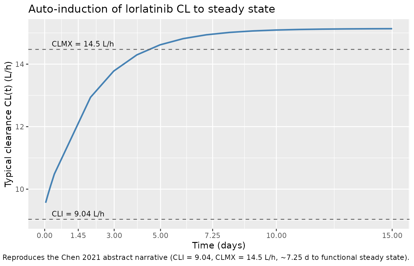
Concentration-time profile at 100 mg q.d.
sim |>
  dplyr::filter(!is.na(Cc), Cc > 1e-3) |>  # log-scale plot; drop pre-first-dose zeros only
  dplyr::group_by(time, treatment) |>
  dplyr::summarise(
    Q05 = quantile(Cc, 0.05, na.rm = TRUE),
    Q50 = quantile(Cc, 0.50, na.rm = TRUE),
    Q95 = quantile(Cc, 0.95, na.rm = TRUE),
    .groups = "drop"
  ) |>
  ggplot(aes(time / 24, Q50, color = treatment, fill = treatment)) +
  geom_ribbon(aes(ymin = Q05, ymax = Q95), alpha = 0.2, color = NA) +
  geom_line(linewidth = 0.7) +
  scale_y_log10() +
  facet_wrap(~treatment, scales = "free_y") +
  labs(x = "Time (days)", y = "Lorlatinib plasma concentration Cc (ng/mL)",
       title = "Simulated plasma concentration profiles",
       caption = "Median and 5th-95th percentile ribbon over 100 virtual subjects per arm.") +
  theme(legend.position = "none")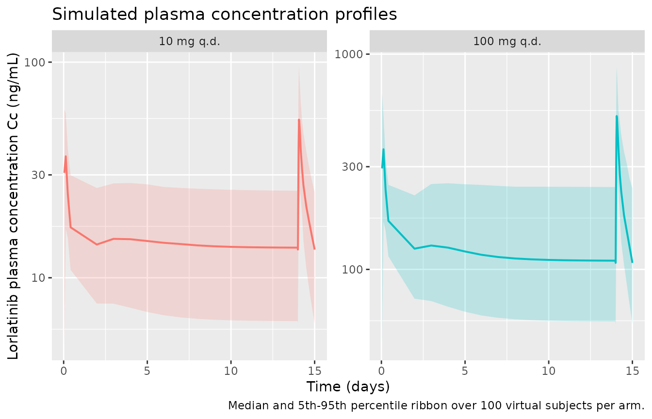
PKNCA validation at steady state
Chen 2021 Methods (“Sensitivity analysis of covariate effects on exposure”) defines the reference typical individual (70 kg, no PPI, WNCL = 100 mL/min, BALB = 4 g/dL, 100 mg q.d.) as having steady-state Cmax = 606 ng/mL and AUCtau = 5180 ng.h/mL over the last (day 15) dosing interval. The PKNCA validation below reproduces these steady-state exposure metrics from the virtual cohort at 100 mg q.d.
# PKNCA input: use ONLY !is.na(Cc) so the time-zero row is preserved.
sim_nca <- sim |>
  dplyr::filter(!is.na(Cc)) |>
  dplyr::select(id, time, Cc, treatment)

# Defensive time-zero row per (id, treatment). Extravascular pre-dose = 0.
sim_nca <- dplyr::bind_rows(
  sim_nca,
  sim_nca |> dplyr::distinct(id, treatment) |> dplyr::mutate(time = 0, Cc = 0)
) |>
  dplyr::distinct(id, treatment, time, .keep_all = TRUE) |>
  dplyr::arrange(id, treatment, time)

conc_obj <- PKNCA::PKNCAconc(
  sim_nca, Cc ~ time | treatment + id,
  concu = "ng/mL", timeu = "h"
)

dose_df <- events |>
  dplyr::filter(evid == 1L) |>
  dplyr::select(id, time, amt, treatment)

dose_obj <- PKNCA::PKNCAdose(
  dose_df, amt ~ time | treatment + id,
  doseu = "mg"
)

# Steady-state interval: the last dosing interval (day 14 to day 15).
last_dose <- max(dose_df$time)
end_ss    <- last_dose + tau

intervals <- data.frame(
  start   = last_dose,
  end     = end_ss,
  cmax    = TRUE,
  tmax    = TRUE,
  auclast = TRUE,
  cav     = TRUE,
  ctrough = TRUE
)

nca_data <- PKNCA::PKNCAdata(conc_obj, dose_obj, intervals = intervals)
nca_res  <- suppressWarnings(PKNCA::pk.nca(nca_data))
Comparison against the published typical-individual exposure
# Published typical-individual exposure at 100 mg q.d. (Chen 2021 Methods
# 'Sensitivity analysis of covariate effects on exposure'). Chen 2021 does
# not report a published 10 mg q.d. Cmax/AUCtau in the Results text; only
# the 100 mg q.d. row can be cross-checked.
published <- tibble::tribble(
  ~treatment,     ~cmax, ~auclast, ~tmax,
  "100 mg q.d.",   606,  5180,     2.0
)

cmp <- nlmixr2lib::ncaComparisonTable(
  simulated     = nca_res,
  reference     = published,
  by            = "treatment",
  units         = c(cmax = "ng/mL", auclast = "ng*h/mL", tmax = "h"),
  tolerance_pct = 25
)

knitr::kable(
  cmp,
  caption = "Simulated (median across 100 virtual subjects) vs. Chen 2021 typical-individual steady-state exposure at 100 mg q.d. Rows differing from reference by >25% receive a trailing asterisk. AUC0-tau over the day 14-15 dosing interval is compared with the paper's `AUCtau` because the model's continuous-CL formulation and stochastic residual error do not target the exact typical-value trajectory the paper's forest-plot simulation reported."
)| NCA parameter | treatment | Reference | Simulated | % diff |
|---|---|---|---|---|
| Cmax (ng/mL) | 100 mg q.d. | 606 | 540 | -11.0% |
| Tmax (h) | 100 mg q.d. | 2 | 1.5 | -25.0% |
| AUClast (ng*h/mL) | 100 mg q.d. | 5180 | 5300 | +2.4% |
Steady-state summary at both doses
nca_tbl <- as.data.frame(nca_res$result) |>
  dplyr::filter(PPTESTCD %in% c("cmax", "auclast", "tmax", "cav", "ctrough")) |>
  dplyr::group_by(treatment, PPTESTCD) |>
  dplyr::summarise(
    median = median(PPORRES, na.rm = TRUE),
    q05    = quantile(PPORRES, 0.05, na.rm = TRUE),
    q95    = quantile(PPORRES, 0.95, na.rm = TRUE),
    .groups = "drop"
  ) |>
  dplyr::mutate(
    Parameter = dplyr::recode(PPTESTCD,
                              cmax    = "Cmax,ss (ng/mL)",
                              auclast = "AUC0-tau,ss (ng*h/mL)",
                              tmax    = "Tmax,ss (h)",
                              cav     = "Cavg,ss (ng/mL)",
                              ctrough = "Ctrough,ss (ng/mL)"),
    median = signif(median, 3),
    q05    = signif(q05, 3),
    q95    = signif(q95, 3)
  ) |>
  dplyr::select(treatment, Parameter, median, q05, q95) |>
  dplyr::rename(
    "Treatment"          = treatment,
    "NCA parameter"      = Parameter,
    "Median"             = median,
    "5th percentile"     = q05,
    "95th percentile"    = q95
  )

knitr::kable(
  nca_tbl,
  caption = "Simulated steady-state NCA distribution over the day 14-15 dosing interval."
)| Treatment | NCA parameter | Median | 5th percentile | 95th percentile |
|---|---|---|---|---|
| 10 mg q.d. | AUC0-tau,ss (ng*h/mL) | 597.0 | 323.0 | 1010.0 |
| 10 mg q.d. | Cavg,ss (ng/mL) | 24.9 | 13.4 | 42.0 |
| 10 mg q.d. | Cmax,ss (ng/mL) | 55.1 | 26.6 | 97.7 |
| 10 mg q.d. | Ctrough,ss (ng/mL) | NA | NA | NA |
| 10 mg q.d. | Tmax,ss (h) | 1.5 | 1.5 | 4.0 |
| 100 mg q.d. | AUC0-tau,ss (ng*h/mL) | 5300.0 | 3310.0 | 8960.0 |
| 100 mg q.d. | Cavg,ss (ng/mL) | 221.0 | 138.0 | 373.0 |
| 100 mg q.d. | Cmax,ss (ng/mL) | 540.0 | 265.0 | 880.0 |
| 100 mg q.d. | Ctrough,ss (ng/mL) | NA | NA | NA |
| 100 mg q.d. | Tmax,ss (h) | 1.5 | 1.5 | 6.0 |
Assumptions and deviations
-
Continuous auto-induction canonical form vs Chen 2021
piecewise SD-flag implementation. Chen 2021 estimated the
auto-induction parameters using a hard NONMEM switch on the SD
(single-dose) data-column flag:
CL = CLIwhenSD = 1, andCL = CLMX * (1 - exp(-IND * TIME))whenSD = 0(NONMEM ListS1 line 63-64). This file implements the continuous canonical form the paper’s narrative describes:CL(t) = CLI + (CLMX - CLI) * (1 - exp(-k_ind * t)), rising smoothly from CLI at t = 0 (first-dose regime) to CLMX at t -> infinity (steady state). The two forms are numerically equivalent at the paper’s estimation anchors (single-dose CL at t = 0 and post-day-15 steady-state CL, whereexp(-0.020 * 336) < 0.002); the continuous form additionally supports arbitrary dosing histories in downstream simulation without requiring a SD covariate column. -
Baseline serum albumin unit conversion. Chen 2021
reports the paper’s
theta_BALB_on_CL = 0.067 per g/dLcentered at BALB = 4 g/dL (the US clinical-lab unit for albumin). The canonical nlmixr2lib covariateALBis in g/L (SI). The model file rescales the coefficient by a factor of 10 (e_alb_cl = 0.00670 per g/L) and centers at 40 g/L. The rescaled term reproduces the paper’s +/-5.3% CL shift at the 10th-percentile ALB = 3.2 g/dL = 32 g/L and +/-4% CL shift at the 90th-percentile ALB = 4.6 g/dL = 46 g/L. -
Weight-normalized (WNCL) vs BSA-normalized (CRCL) creatinine
clearance. Chen 2021 derives WNCL from the Cockcroft-Gault BCCL
by weight- normalization:
WNCL = BCCL / (BWT / 70)^0.75(approximate; the paper cites Rhodin et al. 2009 for the exact form and the exponent choice). The canonicalCRCLcolumn in nlmixr2lib holds BSA-normalized creatinine clearance in mL/min/1.73 m^2 (perinst/references/covariate-columns.md). For the reference 70-kg adult with BSA ~ 1.73 m^2, weight-normalized and BSA-normalized creatinine clearance are numerically nearly identical, so theCRCLcolumn with reference 100 mL/min is a compatible substitute. Downstream users applying the model to obese / underweight cohorts should either (a) precompute WNCL exactly per the Chen 2021 derivation and supply it in theCRCLcolumn, or (b) accept the small numerical discrepancy that arises from the BSA-vs-weight normalization when using BSA-normalized CRCL from routine clinical data. -
Route-specific residual error simplified to the oral
route. Chen 2021 fits separate log-scale residual SDs for the
IV route (
theta = 0.115; Study B7461007 absolute-bioavailability arm) and the oral route (theta = 0.438) via a NONMEMIF(ROUT.EQ.28)branch (ListS1 line 77-81). Because the labelled lorlatinib route of administration is oral and the simulation library targets clinical q.d. tablet dosing, this file encodes only the oral residual SD aspropSd = 0.438. The IV residual SD is documented here for reviewers examining absolute-bioavailability scenarios; a future model file could add a route indicator if IV simulation becomes a priority use case. - Inter-occasion variability (IOV) omitted. The Chen 2021 NONMEM control stream ListS1 does not enable an occasion-level $OMEGA block, so no IOV is encoded here.
- Covariate joint distribution assumed independent. Chen 2021 Table 3 reports the marginal distributions of each covariate but not their joint distribution. The virtual cohort in this vignette samples WT, ALB, CRCL, and CONMED_PPI independently from their marginals; downstream users who need to preserve the empirical BWT-BSA-CRCL correlation observed in real clinical cohorts should either digitize the covariate correlation matrix from a separate source or perform copula-based sampling.
- B7461001 phase I dose-escalation regimens (10-200 mg q.d. and 35-100 mg b.i.d.) are not exercised in the vignette. The illustrative simulation above uses only the 100 mg q.d. labelled dose and a 10 mg q.d. low-end contrast; the full escalation grid is best exercised via a parametric sweep in a downstream simulation script, not embedded in the vignette narrative.