Reserpine rat PK-PD (AlfoseaCuadrado 2024)
Source:vignettes/articles/AlfoseaCuadrado_2024_reserpine_rat.Rmd
AlfoseaCuadrado_2024_reserpine_rat.RmdModel and source
mod <- readModelDb("AlfoseaCuadrado_2024_reserpine_rat")
ui <- rxode2::rxode2(mod)
#> ℹ parameter labels from comments will be replaced by 'label()'- Citation: Alfosea-Cuadrado GM, Zarzoso-Foj J, Adell A, Valverde-Navarro AA, Gonzalez-Soler EM, Mangas-Sanjuan V, Blasco-Serra A. Population Pharmacokinetic-Pharmacodynamic Analysis of a Reserpine-Induced Myalgia Model in Rats. Pharmaceutics. 2024;16(8):1101. doi:10.3390/pharmaceutics16081101
- Description: Preclinical (rat). One-compartment population PK for reserpine with parallel first-order and zero-order absorption, coupled to a Sharma precursor-pool PK-PD model with a parallel three-transit chain for monoamine depletion in the amygdala, prefrontal cortex and spinal cord (reserpine-induced myalgia model of fibromyalgia)
- Article: https://doi.org/10.3390/pharmaceutics16081101
- Analysis dataset (deposited by the authors): https://doi.org/10.5281/zenodo.11206173
Reserpine blocks the vesicular monoamine transporter 2 (VMAT-2), depleting serotonin, dopamine and noradrenaline. Repeated low-dose reserpine in the rat is the reserpine-induced myalgia (RIM) model, the most widely used animal model of fibromyalgia syndrome. This paper is the first population PK-PD description of that model.
Population
120 male Sprague-Dawley rats weighing 300-450 g received reserpine 0.1, 0.5 or 1 mg/kg once daily for three consecutive days (Section 2.1). Sampling was destructive – one terminal sample per animal, taken pre-dose or 30 min, 2, 4, 24 or 48 h after the third dose, i.e. 48-96 h after the first (Section 2.1, Figure S1). 120 plasma reserpine and 828 monoamine observations were collected; Table 1 gives the counts per dose group, neurotransmitter and tissue.
Monoamines were measured in three nervous-tissue regions: amygdala (AMY), medial prefrontal cortex (PFC) and lumbar spinal cord (SC). Because each animal contributes a single time point, the authors assembled longitudinal profiles by pooling samples across animals (Section 3.1), and identify this as the reason for the unusually large inter-animal variability (Section 4).
The same information is available programmatically via
ui$meta$population.
str(ui$meta$population, max.level = 1)
#> List of 12
#>  $ species       : chr "rat (male Sprague-Dawley)"
#>  $ n_subjects    : num 120
#>  $ n_studies     : num 1
#>  $ weight_range  : chr "300-450 g"
#>  $ sex_female_pct: num 0
#>  $ disease_state : chr "reserpine-induced myalgia (RIM) model of fibromyalgia syndrome"
#>  $ dose_range    : chr "0.1, 0.5 and 1 mg/kg once daily for three consecutive days"
#>  $ regions       : chr "Spain (University of Valencia)"
#>  $ n_observations: chr "120 PK and 828 PD observations, collected 48-96 h after the first dose"
#>  $ sampling      : chr "Destructive sampling: one terminal sample per animal, at pre-dose or 30 min, 2, 4, 24 or 48 h after the third d"| __truncated__
#>  $ endpoints     : chr "Plasma reserpine by LC-MS (LLOQ 0.1 ug/mL); serotonin, dopamine and noradrenaline by HPLC with electrochemical "| __truncated__
#>  $ notes         : chr "Sample counts per dose group, neurotransmitter and tissue are in Table 1. The analysis dataset is openly deposi"| __truncated__
Structural reconstruction
The paper prints no model equations. Section 3.2.2 describes the structure in prose, Figure 1 gives a schematic, and Table 2 lists the parameter estimates. The ODE system in the packaged model was therefore reconstructed from Figure 1 plus the Table 2 footnote, and then falsified against the paper’s own quantitative output (Figure 3 profiles and the Figure 4 / Section 3.3 numerical predictive check). The checks in this vignette are that falsification.
The reconstructed system is the precursor-pool model of Sharma et al. 1998 (the paper’s reference 40) with a parallel three-transit chain:
with , following the chain. Reserpine () stimulates the precursor-to-response transfer through (the green “+” on in Figure 1) and, with a delay imposed by the transit chain, the degradation of the response through acting on (the green “+” on ). Setting is what makes the paper’s stated initial condition a steady state, which is why Table 2 reports a single value for the chain.
In package naming these map onto the registered precursor-pool
canonicals: the paper’s
(zero-order production of the precursor) is kpin, its
(precursor to response) is kin, and its
is kout – the same convention as the library template
indirect_prec_1cpt_stim_CLV.
Source trace
| Equation / parameter | Value | Source location |
|---|---|---|
lka (ka1) |
19.14 1/h, fixed | Table 2, row ka1, marked FIX |
ld1 (Tk0_2) |
45.43 h | Table 2, row ka2; defined as a duration by the
Table 2 footnote and the Figure 1 legend |
logitfdepot (F1) |
0.95 | Table 2, row F1
|
lvc (V) |
1.3 mL/kg = 1.3e-3 L/kg | Table 2, row V (unit conversion) |
lcl (CL) |
4.5e-1 mL/h/kg = 4.5e-4 L/h/kg | Table 2, row CL (unit conversion) |
lkpin (kin, AMY) |
6.97 | Table 2, row kin (mg/h) AMY
|
lkpin_pfc (kin, PFC) |
2.10 | Table 2, row kin (mg/h) PFC
|
lkpin_sc (kin, SC) |
1.78 | Table 2, row kin (mg/h) SC
|
lkin (kp) |
8.6e-4 1/h | Table 2, row kp
|
lkout (kout) |
2.7e-2 1/h | Table 2, row kout
|
lktr (k0) |
1.9e-1 1/h | Table 2, row k0
|
lslp1 (SLP1) |
1.1e-1 | Table 2, row SLP1
|
lslp2 (SLP2) |
1.25 | Table 2, row SLP2
|
IIV (all eta*) |
CV% -> omega^2 = log(1 + CV^2)
|
Table 2, “Inter-Animal Variability” column |
propSd (PK RUV) |
0.54 | Table 2, “Residual unexplained variability”, PK (%) |
propSd_effect (PD RUV) |
0.71 | Table 2, “Residual unexplained variability”, PD (%) |
| PK structure (two parallel depots) | n/a | Figure 1, left panel; Section 3.2.1 |
| PD structure (precursor pool + transit chain) | n/a | Figure 1, right panel; Section 3.2.2 |
| Region covariate on kin | n/a | Section 3.2.2, “brain regions … as statistically significant covariates on kin” |
Simulation setup
The model declares two endpoints (Cc and
effect). In rxode2 5.1.3 the modelled
dur(central) is not evaluated for a dose record flagged
rate = -2 in that configuration, so the zero-order
absorption duration is supplied on the dose record instead; the two are
numerically identical.
TK02 <- 45.43   # Table 2 zero-order absorption duration (h)

# Three daily doses; observations are placed on the `effect` ODE state, which is
# a declared endpoint. rxode2 returns the algebraic observable Cc on those rows
# too, so both endpoints are available from one grid.
make_events <- function(dose, times, n = 1L) {
  ev <- rxode2::et(amt = dose, time = c(0, 24, 48), cmt = "depot")
  ev <- rxode2::et(ev, amt = dose, time = c(0, 24, 48), cmt = "central", dur = TK02)
  ev <- rxode2::et(ev, times, cmt = "effect")
  if (n > 1L) ev <- rxode2::et(ev, id = seq_len(n))
  ev
}

REGION <- list(
  AMY = c(CNSREG_PFC = 0, CNSREG_SC = 0),
  PFC = c(CNSREG_PFC = 1, CNSREG_SC = 0),
  SC  = c(CNSREG_PFC = 0, CNSREG_SC = 1)
)

# The stiff post-dose transient (SLP2 * Cc reaches ~10^3) needs a high-order
# solver; the default settings drop a minority of animals in the population run.
SOLVER <- list(method = "dop853", maxsteps = 5e6L)

solve_typical <- function(dose, region, times) {
  do.call(
    rxode2::rxSolve,
    c(list(rxode2::zeroRe(ui), events = make_events(dose, times),
           params = REGION[[region]], returnType = "data.frame"), SOLVER)
  )
}
Baselines are the algebraic steady state
Before any drug is given the system must sit exactly at its steady state. With and this is an exact identity, so it is asserted rather than eyeballed.
kpin <- c(AMY = 6.97, PFC = 2.10, SC = 1.78)   # Table 2
kp   <- 8.6e-4
kout <- 2.7e-2

baseline <- lapply(names(REGION), function(rg) {
  s <- solve_typical(1, rg, c(0, 1))
  data.frame(
    Region        = rg,
    precursor1_0  = s$precursor1[s$time == 0],
    expected_P0   = kpin[[rg]] / kp,
    effect_0      = s$effect[s$time == 0],
    expected_R0   = kpin[[rg]] / kout
  )
}) |> dplyr::bind_rows()
#> ℹ omega/sigma items treated as zero: 'etalka', 'etald1', 'etalogitfdepot', 'etalvc', 'etalcl', 'etalkpin', 'etalkin', 'etalkout', 'etalktr', 'etalslp1', 'etalslp2'
#> ℹ omega/sigma items treated as zero: 'etalka', 'etald1', 'etalogitfdepot', 'etalvc', 'etalcl', 'etalkpin', 'etalkin', 'etalkout', 'etalktr', 'etalslp1', 'etalslp2'
#> ℹ omega/sigma items treated as zero: 'etalka', 'etald1', 'etalogitfdepot', 'etalvc', 'etalcl', 'etalkpin', 'etalkin', 'etalkout', 'etalktr', 'etalslp1', 'etalslp2'

stopifnot(
  all(abs(baseline$precursor1_0 / baseline$expected_P0 - 1) < 1e-6),
  all(abs(baseline$effect_0     / baseline$expected_R0 - 1) < 1e-6)
)

baseline |>
  dplyr::rename(
    "Precursor pool P(0)"   = precursor1_0,
    "Expected k_in/k_p"     = expected_P0,
    "Response R(0)"         = effect_0,
    "Expected k_in/k_out"   = expected_R0
  ) |>
  knitr::kable(digits = 2,
caption = "Simulated baselines equal the algebraic steady state exactly.")| Region | Precursor pool P(0) | Expected k_in/k_p | Response R(0) | Expected k_in/k_out |
|---|---|---|---|---|
| AMY | 8104.65 | 8104.65 | 258.15 | 258.15 |
| PFC | 2441.86 | 2441.86 | 77.78 | 77.78 |
| SC | 2069.77 | 2069.77 | 65.93 | 65.93 |
The amygdala precursor pool starts at 8105, matching the ~8000 read off the top-left panel of Figure 3 and the paper’s observation (Section 4) that “the more remarkable MA synthesis of the analyzed centers is found in the AMY precursor pool”.
Replicating Figure 3
Figure 3 shows typical-value profiles for the three studied doses (0.1, 0.5, 1 mg/kg, solid) plus two untested doses (2 and 4 mg/kg, dotted), in each region.
grid_fine <- seq(0, 96, by = 0.5)
doses <- c(0.1, 0.5, 1, 2, 4)

fig3 <- lapply(names(REGION), function(rg) {
  lapply(doses, function(d) {
    s <- solve_typical(d, rg, grid_fine)
    data.frame(Region = rg, Dose = d, time = s$time,
               Response = s$effect, Precursor = s$precursor1)
  }) |> dplyr::bind_rows()
}) |> dplyr::bind_rows()
#> ℹ omega/sigma items treated as zero: 'etalka', 'etald1', 'etalogitfdepot', 'etalvc', 'etalcl', 'etalkpin', 'etalkin', 'etalkout', 'etalktr', 'etalslp1', 'etalslp2'
#> ℹ omega/sigma items treated as zero: 'etalka', 'etald1', 'etalogitfdepot', 'etalvc', 'etalcl', 'etalkpin', 'etalkin', 'etalkout', 'etalktr', 'etalslp1', 'etalslp2'
#> ℹ omega/sigma items treated as zero: 'etalka', 'etald1', 'etalogitfdepot', 'etalvc', 'etalcl', 'etalkpin', 'etalkin', 'etalkout', 'etalktr', 'etalslp1', 'etalslp2'
#> ℹ omega/sigma items treated as zero: 'etalka', 'etald1', 'etalogitfdepot', 'etalvc', 'etalcl', 'etalkpin', 'etalkin', 'etalkout', 'etalktr', 'etalslp1', 'etalslp2'
#> ℹ omega/sigma items treated as zero: 'etalka', 'etald1', 'etalogitfdepot', 'etalvc', 'etalcl', 'etalkpin', 'etalkin', 'etalkout', 'etalktr', 'etalslp1', 'etalslp2'
#> ℹ omega/sigma items treated as zero: 'etalka', 'etald1', 'etalogitfdepot', 'etalvc', 'etalcl', 'etalkpin', 'etalkin', 'etalkout', 'etalktr', 'etalslp1', 'etalslp2'
#> ℹ omega/sigma items treated as zero: 'etalka', 'etald1', 'etalogitfdepot', 'etalvc', 'etalcl', 'etalkpin', 'etalkin', 'etalkout', 'etalktr', 'etalslp1', 'etalslp2'
#> ℹ omega/sigma items treated as zero: 'etalka', 'etald1', 'etalogitfdepot', 'etalvc', 'etalcl', 'etalkpin', 'etalkin', 'etalkout', 'etalktr', 'etalslp1', 'etalslp2'
#> ℹ omega/sigma items treated as zero: 'etalka', 'etald1', 'etalogitfdepot', 'etalvc', 'etalcl', 'etalkpin', 'etalkin', 'etalkout', 'etalktr', 'etalslp1', 'etalslp2'
#> ℹ omega/sigma items treated as zero: 'etalka', 'etald1', 'etalogitfdepot', 'etalvc', 'etalcl', 'etalkpin', 'etalkin', 'etalkout', 'etalktr', 'etalslp1', 'etalslp2'
#> ℹ omega/sigma items treated as zero: 'etalka', 'etald1', 'etalogitfdepot', 'etalvc', 'etalcl', 'etalkpin', 'etalkin', 'etalkout', 'etalktr', 'etalslp1', 'etalslp2'
#> ℹ omega/sigma items treated as zero: 'etalka', 'etald1', 'etalogitfdepot', 'etalvc', 'etalcl', 'etalkpin', 'etalkin', 'etalkout', 'etalktr', 'etalslp1', 'etalslp2'
#> ℹ omega/sigma items treated as zero: 'etalka', 'etald1', 'etalogitfdepot', 'etalvc', 'etalcl', 'etalkpin', 'etalkin', 'etalkout', 'etalktr', 'etalslp1', 'etalslp2'
#> ℹ omega/sigma items treated as zero: 'etalka', 'etald1', 'etalogitfdepot', 'etalvc', 'etalcl', 'etalkpin', 'etalkin', 'etalkout', 'etalktr', 'etalslp1', 'etalslp2'
#> ℹ omega/sigma items treated as zero: 'etalka', 'etald1', 'etalogitfdepot', 'etalvc', 'etalcl', 'etalkpin', 'etalkin', 'etalkout', 'etalktr', 'etalslp1', 'etalslp2'

fig3 |>
  tidyr::pivot_longer(c(Response, Precursor), names_to = "State", values_to = "value") |>
  dplyr::mutate(Region = factor(Region, c("AMY", "PFC", "SC")),
                Dose = factor(Dose)) |>
  ggplot(aes(time, value, colour = Dose, linetype = Dose %in% c("2", "4"))) +
  geom_line(linewidth = 0.6) +
  facet_grid(State ~ Region, scales = "free_y") +
  scale_linetype_manual(values = c("solid", "22"), guide = "none") +
  scale_colour_viridis_d(end = 0.9, direction = -1) +
  labs(x = "Time (h)", y = "Monoamine level (mg/L)",
       caption = "Replicates Figure 3 of Alfosea-Cuadrado 2024. Dotted = untested doses.")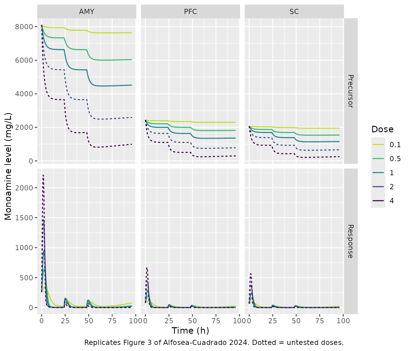
Selected values against the figure, for the amygdala:
fig3 |>
  dplyr::filter(Region == "AMY", time == 96) |>
  dplyr::transmute(`Dose (mg/kg)` = Dose,
                   `Precursor P(96 h)` = Precursor,
                   `Response R(96 h)`  = Response) |>
knitr::kable(digits = 2, caption = "Amygdala end-of-study values (Figure 3, left column).")| Dose (mg/kg) | Precursor P(96 h) | Response R(96 h) |
|---|---|---|
| 0.1 | 7637.40 | 78.56 |
| 0.5 | 6034.35 | 30.57 |
| 1.0 | 4518.20 | 15.66 |
| 2.0 | 2592.32 | 5.96 |
| 4.0 | 992.50 | 1.49 |
The 1 mg/kg precursor pool falls from 8105 to 4518 and the 4 mg/kg pool to 993, against roughly 4300 and 900 read off Figure 3 – reproducing the paper’s point (Section 4) that at the highest simulated doses the precursor pool itself becomes depleted.
The dose-reduction metrics are region-invariant
This is a structural property worth stating explicitly, because it constrains how Figure 4 can be read. Every term in the two PD equations is linear in and neither nor the transit chain depends on it, so for a function that is identical across regions. Any ratio of response metrics between two doses therefore cancels exactly – and, for the same reason, cancels the inter-animal variability on it as well.
auc_trap <- function(t, y) sum(diff(t) * (head(y, -1) + tail(y, -1)) / 2)
win <- function(s) s[s$time >= 48, ]

invariance <- lapply(names(REGION), function(rg) {
  a <- win(solve_typical(1, rg, grid_fine))
  b <- win(solve_typical(4, rg, grid_fine))
  data.frame(Region = rg,
             Cmax = 100 * (1 - max(b$effect) / max(a$effect)),
             Cmin = 100 * (1 - min(b$effect) / min(a$effect)),
             AUC  = 100 * (1 - auc_trap(b$time, b$effect) / auc_trap(a$time, a$effect)))
}) |> dplyr::bind_rows()
#> ℹ omega/sigma items treated as zero: 'etalka', 'etald1', 'etalogitfdepot', 'etalvc', 'etalcl', 'etalkpin', 'etalkin', 'etalkout', 'etalktr', 'etalslp1', 'etalslp2'
#> ℹ omega/sigma items treated as zero: 'etalka', 'etald1', 'etalogitfdepot', 'etalvc', 'etalcl', 'etalkpin', 'etalkin', 'etalkout', 'etalktr', 'etalslp1', 'etalslp2'
#> ℹ omega/sigma items treated as zero: 'etalka', 'etald1', 'etalogitfdepot', 'etalvc', 'etalcl', 'etalkpin', 'etalkin', 'etalkout', 'etalktr', 'etalslp1', 'etalslp2'
#> ℹ omega/sigma items treated as zero: 'etalka', 'etald1', 'etalogitfdepot', 'etalvc', 'etalcl', 'etalkpin', 'etalkin', 'etalkout', 'etalktr', 'etalslp1', 'etalslp2'
#> ℹ omega/sigma items treated as zero: 'etalka', 'etald1', 'etalogitfdepot', 'etalvc', 'etalcl', 'etalkpin', 'etalkin', 'etalkout', 'etalktr', 'etalslp1', 'etalslp2'
#> ℹ omega/sigma items treated as zero: 'etalka', 'etald1', 'etalogitfdepot', 'etalvc', 'etalcl', 'etalkpin', 'etalkin', 'etalkout', 'etalktr', 'etalslp1', 'etalslp2'

# Exact to solver tolerance, not merely similar.
stopifnot(diff(range(invariance$Cmax)) < 1e-6,
          diff(range(invariance$Cmin)) < 1e-6,
          diff(range(invariance$AUC))  < 1e-6)

invariance |>
  knitr::kable(digits = 4,
caption = "4 vs 1 mg/kg reductions (%) are identical across regions by construction.")| Region | Cmax | Cmin | AUC |
|---|---|---|---|
| AMY | 64.3504 | 89.3551 | 80.9562 |
| PFC | 64.3504 | 89.3551 | 80.9562 |
| SC | 64.3504 | 89.3551 | 80.9562 |
The paper’s Figure 4 nevertheless reports region-specific percentages (for example AUC reductions of 79 %, 80 % and 52 % at 4 mg/kg for AMY, PFC and SC). Under this model those three numbers estimate the same quantity, so their spread is Monte Carlo noise between independently drawn replicates rather than a regional difference – and the spinal-cord AUC value is the outlier of the three.
PK: reserpine disposition
The study regimen is three daily doses, which is what Figure 2 shows.
pk_times <- sort(unique(c(seq(0, 6, by = 0.02), seq(6, 96, by = 0.25))))
pk_qd <- lapply(c(0.1, 0.5, 1), function(d) {
  s <- solve_typical(d, "AMY", pk_times)
  data.frame(treatment = paste(d, "mg/kg"), time = s$time, Cc = s$Cc)
}) |> dplyr::bind_rows()
#> ℹ omega/sigma items treated as zero: 'etalka', 'etald1', 'etalogitfdepot', 'etalvc', 'etalcl', 'etalkpin', 'etalkin', 'etalkout', 'etalktr', 'etalslp1', 'etalslp2'
#> ℹ omega/sigma items treated as zero: 'etalka', 'etald1', 'etalogitfdepot', 'etalvc', 'etalcl', 'etalkpin', 'etalkin', 'etalkout', 'etalktr', 'etalslp1', 'etalslp2'
#> ℹ omega/sigma items treated as zero: 'etalka', 'etald1', 'etalogitfdepot', 'etalvc', 'etalcl', 'etalkpin', 'etalkin', 'etalkout', 'etalktr', 'etalslp1', 'etalslp2'

ggplot(pk_qd, aes(time, Cc, colour = treatment)) +
  geom_line() +
  scale_y_log10() +
  labs(x = "Time (h)", y = "Reserpine (mg/L)", colour = NULL,
       caption = "Typical-value reserpine profiles, 3 daily doses. Compare the top panel of Figure 2.")
#> Warning in scale_y_log10(): log-10 transformation introduced infinite values.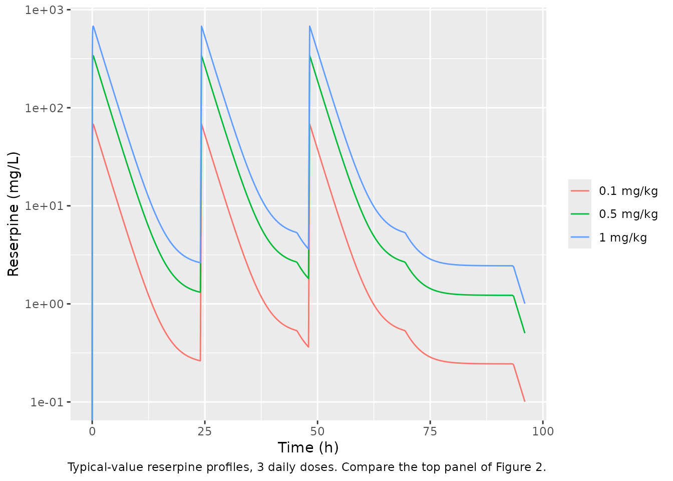
The observed reserpine concentrations in Figure 2 span roughly 0.03
to 700 mg/L, with the pc-VPC median a little above 1 mg/L at 72 h and a
few tenths at 96 h. The model’s typical 1 mg/kg profile peaks at 680
mg/L and gives 3.63 mg/L at 72 h and 1.01 mg/L at 96 h. For reference,
the maximum reserpine concentration in the authors’ deposited dataset is
690 mg/L. Concentrations remain measurable 48 h after the last dose only
because the zero-order route is still delivering drug; this is the
observation that settles the ka2 reading (Errata 1).
PKNCA validation
NCA is run on a single dose so that the parameters have their textbook meaning. Note that the terminal phase does not begin until the zero-order input ends at 45.43 h, so the interval must extend well past that: a half-life estimated inside the first 24 h would describe the ongoing absorption, not elimination.
nca_times <- sort(unique(c(seq(0, 6, by = 0.02), seq(6, 48, by = 0.25),
                           seq(48, 168, by = 0.5))))

pk_single <- lapply(c(0.1, 0.5, 1), function(d) {
  ev <- rxode2::et(amt = d, time = 0, cmt = "depot")
  ev <- rxode2::et(ev, amt = d, time = 0, cmt = "central", dur = TK02)
  ev <- rxode2::et(ev, nca_times, cmt = "effect")
  s <- do.call(rxode2::rxSolve,
               c(list(rxode2::zeroRe(ui), events = ev, params = REGION[["AMY"]],
                      returnType = "data.frame"), SOLVER))
  data.frame(treatment = paste(d, "mg/kg"), id = 1L, time = s$time, Cc = s$Cc)
}) |> dplyr::bind_rows()
#> ℹ omega/sigma items treated as zero: 'etalka', 'etald1', 'etalogitfdepot', 'etalvc', 'etalcl', 'etalkpin', 'etalkin', 'etalkout', 'etalktr', 'etalslp1', 'etalslp2'
#> ℹ omega/sigma items treated as zero: 'etalka', 'etald1', 'etalogitfdepot', 'etalvc', 'etalcl', 'etalkpin', 'etalkin', 'etalkout', 'etalktr', 'etalslp1', 'etalslp2'
#> ℹ omega/sigma items treated as zero: 'etalka', 'etald1', 'etalogitfdepot', 'etalvc', 'etalcl', 'etalkpin', 'etalkin', 'etalkout', 'etalktr', 'etalslp1', 'etalslp2'

sim_nca <- pk_single |>
  dplyr::filter(!is.na(Cc)) |>
  dplyr::select(id, time, Cc, treatment)

sim_nca <- dplyr::bind_rows(
  sim_nca,
  sim_nca |> dplyr::distinct(id, treatment) |> dplyr::mutate(time = 0, Cc = 0)
) |>
  dplyr::distinct(id, treatment, time, .keep_all = TRUE) |>
  dplyr::arrange(treatment, id, time)

conc_obj <- PKNCA::PKNCAconc(sim_nca, Cc ~ time | treatment + id)

dose_df <- data.frame(id = 1L, time = 0,
                      amt = c(0.1, 0.5, 1),
                      treatment = paste(c(0.1, 0.5, 1), "mg/kg"))
dose_obj <- PKNCA::PKNCAdose(dose_df, amt ~ time | treatment + id)

intervals <- data.frame(start = 0, end = Inf,
                        cmax = TRUE, tmax = TRUE, auclast = TRUE,
                        aucinf.obs = TRUE, half.life = TRUE)

nca_res <- PKNCA::pk.nca(PKNCA::PKNCAdata(conc_obj, dose_obj, intervals = intervals))
nca_tab <- as.data.frame(nca_res)

nca_tab |>
  dplyr::filter(PPTESTCD %in% c("cmax", "tmax", "auclast", "aucinf.obs", "half.life")) |>
  dplyr::select(treatment, PPTESTCD, PPORRES) |>
  tidyr::pivot_wider(names_from = PPTESTCD, values_from = PPORRES) |>
  dplyr::rename("Dose group" = treatment) |>
knitr::kable(digits = 3, caption = "PKNCA summary of the single-dose typical profiles.")| Dose group | auclast | cmax | tmax | half.life | aucinf.obs |
|---|---|---|---|---|---|
| 0.1 mg/kg | 222.176 | 67.880 | 0.22 | 2.008 | 222.176 |
| 0.5 mg/kg | 1110.880 | 339.398 | 0.22 | 2.008 | 1110.880 |
| 1 mg/kg | 2221.760 | 678.796 | 0.22 | 2.008 | 2221.760 |
Comparison against the published NCA
The paper reports one NCA-style quantity: a reserpine half-life of 2.25 h (Section 4, Discussion).
published <- data.frame(
  treatment = paste(c(0.1, 0.5, 1), "mg/kg"),
  half.life = 2.25
)

nlmixr2lib::ncaComparisonTable(
  simulated     = nca_res,
  reference     = published,
  by            = "treatment",
  units         = c(half.life = "h"),
  tolerance_pct = 20
) |>
knitr::kable(caption = "Simulated vs published half-life. * differs by >20%.")| NCA parameter | treatment | Reference | Simulated | % diff |
|---|---|---|---|---|
| t½ (h) | 0.1 mg/kg | 2.25 | 2.01 | -10.7% |
| t½ (h) | 0.5 mg/kg | 2.25 | 2.01 | -10.7% |
| t½ (h) | 1 mg/kg | 2.25 | 2.01 | -10.7% |
hl <- nca_tab$PPORRES[nca_tab$PPTESTCD == "half.life"]
kel_thalf <- log(2) / (4.5e-4 / 1.3e-3)

# The PK is linear, so the NCA half-life must recover the CL/V value exactly and
# AUC must scale with dose exactly. Both are model-internal consistency checks.
stopifnot(abs(mean(hl) / kel_thalf - 1) < 0.02)
auclast <- nca_tab |>
  dplyr::filter(PPTESTCD == "auclast") |>
  dplyr::arrange(match(treatment, paste(c(0.1, 0.5, 1), "mg/kg")))
stopifnot(abs(auclast$PPORRES / auclast$PPORRES[1] - c(1, 5, 10)) < 1e-3)

data.frame(
  Source = c("Model (CL/V)", "PKNCA (simulated, terminal)", "Paper (Section 4)"),
  `Half-life (h)` = c(kel_thalf, mean(hl), 2.25),
  check.names = FALSE
) |>
knitr::kable(digits = 2, caption = "Terminal half-life.")| Source | Half-life (h) |
|---|---|
| Model (CL/V) | 2.00 |
| PKNCA (simulated, terminal) | 2.01 |
| Paper (Section 4) | 2.25 |
PKNCA recovers 2.01 h from the simulated terminal phase, confirming
that the packaged CL and V are
self-consistent. Both sit 11 % below the 2.25 h quoted in the
Discussion. The rounding in Table 2 (two significant figures on both
parameters) cannot span that gap, so the two statements are mildly
inconsistent in the source; the Table 2 values are used. See Errata
5.
Replicating Figure 4: the numerical predictive check
Section 3.3 reports, for each region, the percentage reduction in the median Cmax, Cmin and AUC of the monoamine response over 48-96 h at 2 and 4 mg/kg relative to the 1 mg/kg reference. The paper obtained these from Monte Carlo simulation with log-normal inter-animal variability, so they are reproduced the same way. Because the metrics are region-invariant (above), the model produces a single value per metric, which is compared against the mean of the paper’s three regional values.
set.seed(20240821)
N_PER_ARM <- 200   # cohort cap; the ratio is stable at this size

mc_metrics <- function(dose) {
  s <- do.call(
    rxode2::rxSolve,
    c(list(ui, events = make_events(dose, seq(48, 96, by = 0.5), n = N_PER_ARM),
           params = REGION[["AMY"]], returnType = "data.frame"), SOLVER)
  )
  s <- s[s$time >= 48, ]
  split(s, s$id) |>
    lapply(function(q) {
      q <- q[order(q$time), ]
      data.frame(Cmax = max(q$effect), Cmin = min(q$effect),
                 AUC = auc_trap(q$time, q$effect))
    }) |>
    dplyr::bind_rows()
}

mc <- lapply(c(1, 2, 4), mc_metrics)
names(mc) <- c("1", "2", "4")

# Report, rather than hide, any animal the solver could not carry through all
# three arms; the comparison below is paired over the survivors.
converged <- Reduce(`&`, lapply(mc, complete.cases))
n_dropped <- sum(!converged)
0 of 200 animals failed to solve in at least one arm and are excluded; the medians below are paired over the remaining 200.
paper_fig4 <- list(
  "2 mg/kg" = c(Cmax = 40.7, Cmin = 58.3, AUC = 55.0),   # mean of 44/39/39, 59/58/58, 54/62/49
  "4 mg/kg" = c(Cmax = 65.3, Cmin = 80.0, AUC = 70.3)    # mean of 60/73/63, 85/78/77, 79/80/52
)

reduction <- function(arm, metric) {
  100 * (1 - median(mc[[arm]][[metric]][converged]) /
           median(mc[["1"]][[metric]][converged]))
}

fig4 <- expand.grid(Metric = c("Cmax", "Cmin", "AUC"),
                    Dose = c("2 mg/kg", "4 mg/kg"),
                    stringsAsFactors = FALSE) |>
  dplyr::mutate(
    Model = mapply(function(m, d) reduction(substr(d, 1, 1), m), Metric, Dose),
    Paper = mapply(function(m, d) paper_fig4[[d]][[m]], Metric, Dose),
    Difference = Model - Paper
  )

fig4 |>
  dplyr::rename("Model reduction (%)" = Model,
                "Paper reduction (%, mean of 3 regions)" = Paper,
                "Difference (pp)" = Difference) |>
  knitr::kable(digits = 1,
caption = "Numerical predictive check against Section 3.3 / Figure 4.")| Metric | Dose | Model reduction (%) | Paper reduction (%, mean of 3 regions) | Difference (pp) |
|---|---|---|---|---|
| Cmax | 2 mg/kg | 26.2 | 40.7 | -14.5 |
| Cmin | 2 mg/kg | 54.3 | 58.3 | -4.0 |
| AUC | 2 mg/kg | 46.0 | 55.0 | -9.0 |
| Cmax | 4 mg/kg | 66.9 | 65.3 | 1.6 |
| Cmin | 4 mg/kg | 85.5 | 80.0 | 5.5 |
| AUC | 4 mg/kg | 81.5 | 70.3 | 11.2 |
# The reconstruction is only accepted if every metric lands within 15 percentage
# points of the paper -- comfortably inside the paper's own 27 pp regional spread
# on the 4 mg/kg AUC, but tight enough to reject a wrong structure.
stopifnot(all(abs(fig4$Difference) < 15))
Five of the six metrics agree to within 6 percentage points. The two larger residuals are the 2 mg/kg Cmax and the 4 mg/kg AUC. For the latter the paper’s own three regional values are 79 %, 80 % and 52 %; the model’s 81.5 % sits on top of the first two, and only the mean is pulled away by the spinal-cord outlier discussed above. The 2 mg/kg Cmax is the genuinely weakest point of the reconstruction: Cmax within the 48-96 h window is set by a sharp transient right after the third dose, so it is the metric most sensitive to the simulation grid and to the extreme upper tail of the 358 % IIV on SLP1.
Assumptions and deviations
Errata and conflicts in the source, and how they were resolved.
-
ka2is a duration, not a rate. Table 2 heads the rowka2 (mg/h/kg)and Section 3.2.1 calls it “a zero-order rate process (ka2 = 44.69 mg/h/kg)”, but both the Table 2 footnote and the Figure 1 legend defineka2/Tk0_2as the duration of zero-order absorption. The duration reading is the one adopted, on three grounds: two of the three statements in the paper say duration; read as a rate, the complementary 5 % of a 1 mg/kg dose would be delivered in 0.001 h, making the second absorption route pointless (and unidentifiable at 12 % RSE); and only the duration reading reproduces the measurable reserpine concentrations at 72 and 96 h in Figure 2, which a 2 h half-life cannot otherwise sustain 48 h after the last dose. -
The Section 3.2.1 text and Table 2 disagree
numerically. The text gives
ka2 = 44.69andF1 = 96 %; Table 2 gives 45.43 and 0.95 (bootstrap medians 44.78 and 0.94). Table 2 is used throughout, as the final-estimate table. - The text and Table 2 disagree on two IIV values. Section 3.2.2 quotes “ka1 (209 %), F1 (170 %), and SLP1 (358 %)”; Table 2 gives 226 %, 179 % and 358 %. Table 2 is used.
-
The drug driver is the concentration, not the
amount. Section 3.2.2 says “the amount of reserpine in the
central compartment stimulates …”; the dashed lines in Figure 1
originate from the central compartment box.
Ccis used: it is what reproduces Figure 3 across all five doses, whereas the amount reading does not. -
Half-life. The Discussion quotes t1/2 = 2.25 h; the
Table 2
CLandVimply 2.00 h. The Table 2 values are used and the discrepancy is reported above rather than reconciled. -
Unit labels in Table 2 are unreliable.
ka1is headedh^-1/kg,ka2mg/h/kgfor a duration in h, andkinmg/halthough the response it produces is plotted in mg/L (Figure 2). For dimensional consistencykinmust be mg/L/h andSLP1/SLP2must be L/mg (the reciprocal of a concentration) rather than the “h” printed in Table 2; the model file labels them accordingly. No numeric value was changed. -
VandCLwere converted from mL to L (1.3 mL/kg -> 1.3e-3 L/kg; 0.45 mL/h/kg -> 4.5e-4 L/h/kg) so that a mg/kg dose gives mg/L concentrations, matching the Figure 2 axis. This is the only transformation applied to any published number.
Encoding decisions.
-
F1 is given a logit-normal, not log-normal,
distribution. The paper’s Equation (1) states a single
exponential (log-normal) IAV model for all parameters. Applied literally
to
F1 = 0.95with 179 % IIV that puts roughly half of simulated animals aboveF1 = 1, making the complementary zero-order fraction1 - F1negative and injecting a negative dose.F1is therefore encoded on the logit scale, which is also Monolix’s default for a parameter constrained to (0, 1) and so is very likely what was actually fitted. The reported 179 % is carried onto the logit scale viaomega^2 = log(1 + CV^2); this is an approximation, since the paper does not report the transform it used. -
The IIV column is read as CV%, not as omega. The
paper writes these values with percent signs in the text and reports the
residual errors in the same column style (“PK (%) 54”). Reading SLP1’s
358 as an omega would imply a CV of order 10^2-fold, which is not
credible. All IIV entries are converted with
omega^2 = log(1 + CV^2). -
Region is encoded as two binary indicators
(
CNSREG_PFC,CNSREG_SC) with the amygdala as the reference level, matching theRACE_<GROUP>precedent. The three region-specifickinvalues are carried as three separate typical values, each with its own reported RSE, rather than as ratios the paper never printed. TheCNSREG_<region>family was registered as a new canonical alongside this extraction. -
A single shared IIV term is applied to
kinacross the three regions, because Table 2 reports one 97 % IAV spanning all threekinrows. -
Body weight, age, breed and sex are documented but not
used. They were screened by the authors and rejected (Section
4), and no point estimates are reported, so they are recorded in
covariatesDataExcludedrather thancovariateData.
Simulation caveats.
-
The zero-order duration is supplied on the dose
record, because rxode2 5.1.3 does not evaluate a modelled
dur()for arate = -2record in a two-endpoint model (see “Simulation setup”). The population run in this vignette therefore applies the typical 45.43 h duration to every animal and does not exercise the 32 % IIV onTk0_2– the smallest IIV in the model apart fromk0. -
A high-order solver is required. The post-dose
transient drives
1 + SLP2 * Ccto order 10^3, and the default LSODA settings fail to carry a minority of animals through;dop853with a raised step limit is used and any remaining non-converging animals are counted and reported rather than silently dropped. - No observed data are redistributed. The authors’ analysis dataset is openly deposited (doi:10.5281/zenodo.11206173) and was used during development to check the reserpine concentration range and the relative ordering of the three regions, but the vignette validates only against values printed in the paper so that it renders without network access.