Propofol (Wahlquist 2024)
Source:vignettes/articles/Wahlquist_2024_propofol.Rmd
Wahlquist_2024_propofol.Rmd
library(nlmixr2lib)
library(PKNCA)
#>
#> Attaching package: 'PKNCA'
#> The following object is masked from 'package:stats':
#>
#>     filter
library(dplyr)
#>
#> Attaching package: 'dplyr'
#> The following objects are masked from 'package:stats':
#>
#>     filter, lag
#> The following objects are masked from 'package:base':
#>
#>     intersect, setdiff, setequal, union
library(ggplot2)
Overview
Wahlquist, Sundell and Soltesz (2024) introduce a symbolic-regression network method that learns the structure of a pharmacometric covariate model at the same time as its coefficients, instead of selecting covariate functions by hand in a stepwise search. The method is demonstrated on the pooled propofol dataset of Eleveld et al. (2018): 15,433 plasma concentrations from 1,031 individuals in 30 studies, spanning neonates to the elderly.
The demonstration produces a complete, fully specified
three-compartment propofol PK model (the paper’s Eq. 10), and that is
what this vignette validates. The learned covariate model is unusual for
pharmacometrics: it maps covariates to the micro rate constants
through low-order polynomials and ratios of polynomials rather than
through the customary multiplicative
TV * (COV/ref)^exponent form, and it uses only three of the
five candidate covariates (age, weight, BMI, plus a sex switch); blood
sampling site was pruned away automatically.
The model is deterministic. It was fitted by minimising the mean median absolute logarithmic error (MdALE, Eqs. 5 and 6) with gradient descent, not by maximum likelihood, so there are no random effects, no standard errors, and no residual-error model to extract.
Population
mod <- readModelDb("Wahlquist_2024_propofol")
pop <- rxode2::rxode2(mod)$meta$population
tibble::tibble(Field = names(pop), Value = vapply(pop, as.character, character(1))) |>
knitr::kable(caption = "Population metadata (Data set section and Table 1).")| Field | Value |
|---|---|
| species | human |
| n_subjects | 1031 |
| n_studies | 30 |
| age_range | 27 weeks postmenstrual to 88 years |
| weight_range | 0.68-160 kg |
| bmi_range | 6.2-52.8 kg/m^2 |
| sex_female_pct | 35 |
| disease_state | surgical and volunteer cohorts receiving propofol for sedation or general anaesthesia |
| dose_range | intravenous bolus and infusion regimens as administered in the 30 pooled studies |
| notes | The pooled dataset published by Eleveld et al. (2018) doi:10.1016/j.bja.2018.01.018, comprising 15,433 plasma concentration observations (11,530 arterial, 3,903 venous) from 1,031 individuals (670 male, 361 female) in 30 clinical studies. Eleveld’s original release holds 1,033 individuals; two were excluded here for having no observations (Data set section, footnote 1). Table 1 lists the covariate ranges. |
The 1,031 individuals comprise 670 males and 361 females. Covariate ranges (Table 1) are age 0-88 years (the text gives 27 weeks postmenstrual as the lower bound), weight 0.68-160 kg, and BMI 6.2-52.8 kg/m^2. Of the observations, 11,530 were arterial and 3,903 venous.
Source trace
tibble::tribble(
  ~Quantity, ~Source,
  "Three-compartment mammillary ODE system", "Eq. 1 (a-c), written for xi = Ai / V1",
  "V1/V2/V3 and CL/Q2/Q3 conversions", "Eq. 2 (a-e)",
  "Final-layer base expression g3(z3) = |z3|", "Eq. 8",
  "k10 = 0.00441 (WGT/WGTmax) + 0.00342", "Eq. 10a",
  "k12 numerator and denominator coefficients", "Eq. 10b",
  "k12 network-output normalisation 0.013328808", "Reference-27 code deposit (see Errata)",
  "k13 male (age-linear terms positive)", "Eq. 10c",
  "k13 female (age-linear terms negative)", "Eq. 10d",
  "k21 coefficients", "Eq. 10e",
  "k31 male / female", "Eqs. 10f / 10g",
  "V1 coefficients", "Eq. 10h",
  "AGEmax 88 y, WGTmax 160 kg, BMImax 52.8 kg/m^2", "Results text following Eq. 10",
  "BMImax full precision 52.84713965", "Reference-27 code deposit (get_results.jl)",
  "Population, covariate ranges, observation counts", "Data set section; Table 1",
  "MdALE / MdLE / MdAPE / MdPE model comparison", "Table 2"
) |>
knitr::kable(caption = "Source location for every equation and ini() value.")| Quantity | Source |
|---|---|
| Three-compartment mammillary ODE system | Eq. 1 (a-c), written for xi = Ai / V1 |
| V1/V2/V3 and CL/Q2/Q3 conversions | Eq. 2 (a-e) |
| Final-layer base expression g3(z3) = |z3| | Eq. 8 |
| k10 = 0.00441 (WGT/WGTmax) + 0.00342 | Eq. 10a |
| k12 numerator and denominator coefficients | Eq. 10b |
| k12 network-output normalisation 0.013328808 | Reference-27 code deposit (see Errata) |
| k13 male (age-linear terms positive) | Eq. 10c |
| k13 female (age-linear terms negative) | Eq. 10d |
| k21 coefficients | Eq. 10e |
| k31 male / female | Eqs. 10f / 10g |
| V1 coefficients | Eq. 10h |
| AGEmax 88 y, WGTmax 160 kg, BMImax 52.8 kg/m^2 | Results text following Eq. 10 |
| BMImax full precision 52.84713965 | Reference-27 code deposit (get_results.jl) |
| Population, covariate ranges, observation counts | Data set section; Table 1 |
| MdALE / MdLE / MdAPE / MdPE model comparison | Table 2 |
Representative subjects
The model has no inter-individual variability, so a subject is fully determined by its covariates. Six subjects spanning the covariate ranges of Table 1 are used throughout.
cohort <- tibble::tribble(
  ~id, ~subject,          ~AGE,  ~WT,  ~BMI, ~SEXF,
  1L,  "Neonate",         0.08,   3.5, 13.0,     0,
  2L,  "Child",           5.00,  20.0, 15.6,     0,
  3L,  "Adult male",     35.00,  70.0, 24.2,     0,
  4L,  "Adult female",   35.00,  70.0, 24.2,     1,
  5L,  "Obese adult",    50.00, 120.0, 39.2,     0,
  6L,  "Elderly",        80.00,  70.0, 25.7,     0
)
cohort |> knitr::kable(caption = "Representative subjects, all inside the Table 1 covariate ranges.")| id | subject | AGE | WT | BMI | SEXF |
|---|---|---|---|---|---|
| 1 | Neonate | 0.08 | 3.5 | 13.0 | 0 |
| 2 | Child | 5.00 | 20.0 | 15.6 | 0 |
| 3 | Adult male | 35.00 | 70.0 | 24.2 | 0 |
| 4 | Adult female | 35.00 | 70.0 | 24.2 | 1 |
| 5 | Obese adult | 50.00 | 120.0 | 39.2 | 0 |
| 6 | Elderly | 80.00 | 70.0 | 25.7 | 0 |
The model reports the individual rate constants and volume as derived quantities, so they can be read directly out of a solve.
param_at_zero <- function(covs) {
  ev <- rxode2::et(0, cmt = "central")
  d <- as.data.frame(ev)
  d <- d[rep(1, nrow(covs)), , drop = FALSE]
  d$id <- covs$id
  d$AGE <- covs$AGE
  d$WT <- covs$WT
  d$BMI <- covs$BMI
  d$SEXF <- covs$SEXF
  s <- rxode2::rxSolve(mod, events = d, returnType = "data.frame")
  s[!duplicated(s$id), c("id", "kel", "k12", "k21", "k13", "k31", "vc")]
}

pk <- param_at_zero(cohort) |>
  dplyr::left_join(cohort[, c("id", "subject")], by = "id") |>
  dplyr::mutate(
    CL = kel * vc * 60,
    Q2 = k12 * vc * 60,
    Q3 = k13 * vc * 60,
    V1 = vc,
    V2 = k12 / k21 * vc,
    V3 = k13 / k31 * vc,
    Vss = V1 + V2 + V3
  )
#> Warning: multi-subject simulation without without 'omega'

pk |>
  dplyr::select(subject, V1, V2, V3, Vss, CL, Q2, Q3) |>
  dplyr::rename(
    "Subject" = subject, "V1 (L)" = V1, "V2 (L)" = V2, "V3 (L)" = V3,
    "Vss (L)" = Vss, "CL (L/min)" = CL, "Q2 (L/min)" = Q2, "Q3 (L/min)" = Q3
  ) |>
  knitr::kable(digits = 2,
caption = "Volumes and clearances derived from the learned rate constants via Eq. 2.")| Subject | V1 (L) | V2 (L) | V3 (L) | Vss (L) | CL (L/min) | Q2 (L/min) | Q3 (L/min) |
|---|---|---|---|---|---|---|---|
| Neonate | 0.35 | 0.53 | 33.15 | 34.03 | 0.07 | 0.07 | 0.09 |
| Child | 2.05 | 3.31 | 181.70 | 187.06 | 0.49 | 0.41 | 0.50 |
| Adult male | 4.92 | 11.04 | 283.24 | 299.21 | 1.58 | 1.01 | 0.90 |
| Adult female | 4.92 | 11.04 | 546.70 | 562.66 | 1.58 | 1.01 | 1.23 |
| Obese adult | 4.81 | 25.54 | 236.40 | 266.74 | 1.94 | 0.99 | 0.80 |
| Elderly | 4.17 | 9.90 | 163.76 | 177.83 | 1.34 | 0.91 | 0.62 |
The paper states in the Discussion that “the obtained values of individual volumes and clearances were comparable to those in [4]”. The reference patient of Eleveld et al. (2018) is a 35-year-old, 70 kg, 1.7 m male, with V1 6.28 L, V2 25.5 L, V3 273 L, CL 1.79 L/min, Q2 1.75 L/min and Q3 1.11 L/min. The “Adult male” row above is the matching subject.
ref <- pk[pk$subject == "Adult male", ]
tibble::tribble(
  ~Parameter,      ~Symreg,      ~Eleveld,
  "V1 (L)",        ref$V1,       6.28,
  "V2 (L)",        ref$V2,       25.5,
  "V3 (L)",        ref$V3,       273,
  "Vss (L)",       ref$Vss,      6.28 + 25.5 + 273,
  "CL (L/min)",    ref$CL,       1.79,
  "Q2 (L/min)",    ref$Q2,       1.75,
  "Q3 (L/min)",    ref$Q3,       1.11
) |>
  dplyr::mutate(`Ratio` = Symreg / Eleveld) |>
  dplyr::rename("Symbolic regression" = Symreg, "Eleveld 2018 reference patient" = Eleveld) |>
  knitr::kable(digits = 2,
caption = "Reference-patient comparison against Eleveld et al. (2018).")| Parameter | Symbolic regression | Eleveld 2018 reference patient | Ratio |
|---|---|---|---|
| V1 (L) | 4.92 | 6.28 | 0.78 |
| V2 (L) | 11.04 | 25.50 | 0.43 |
| V3 (L) | 283.24 | 273.00 | 1.04 |
| Vss (L) | 299.21 | 304.78 | 0.98 |
| CL (L/min) | 1.58 | 1.79 | 0.88 |
| Q2 (L/min) | 1.01 | 1.75 | 0.58 |
| Q3 (L/min) | 0.90 | 1.11 | 0.81 |
Steady-state volume and clearance agree closely (Vss within 2%, CL within 12%). The split between the two peripheral compartments differs: the symbolic regression puts less drug in the shallow compartment and slightly more in the deep one. This is expected – the ALE loss constrains the predicted concentration profile, not the individual compartment volumes, which are only weakly identifiable.
Simulation of a single intravenous bolus
Propofol is given intravenously, so all doses go directly into
central. Time is in seconds throughout, matching the
published rate constants.
dose_mg_per_kg <- 2
tgrid <- unique(c(seq(0, 300, by = 10), seq(300, 3600, by = 60),
                  seq(3600, 86400, by = 900)))

build_events <- function(covs, mgkg) {
  do.call(rbind, lapply(seq_len(nrow(covs)), function(i) {
    r <- covs[i, ]
    d <- data.frame(
      id = r$id,
      time = c(0, tgrid),
      amt = c(r$WT * mgkg, rep(NA_real_, length(tgrid))),
      evid = c(1L, rep(0L, length(tgrid))),
      cmt = "central"
    )
    d$AGE <- r$AGE; d$WT <- r$WT; d$BMI <- r$BMI; d$SEXF <- r$SEXF
    d$subject <- r$subject
    d$dose_mg <- r$WT * mgkg
    d
  }))
}

ev <- build_events(cohort, dose_mg_per_kg)
# Tight integration tolerances: the dose-linearity gate below compares two
# ODE-integrated solves to 1e-6, which the defaults (rtol 1e-6, atol 1e-8)
# cannot deliver.
sim <- rxode2::rxSolve(mod, events = ev, keep = c("subject", "dose_mg"),
                       returnType = "data.frame", rtol = 1e-10, atol = 1e-12)
#> Warning: multi-subject simulation without without 'omega'
sim |>
  dplyr::filter(time > 0, time <= 14400, Cc > 0) |>
  ggplot(aes(time / 60, Cc, colour = subject)) +
  geom_line(linewidth = 0.7) +
  scale_y_log10() +
  labs(x = "Time (min)", y = "Plasma propofol (mg/L = ug/mL)", colour = NULL) +
  theme_bw()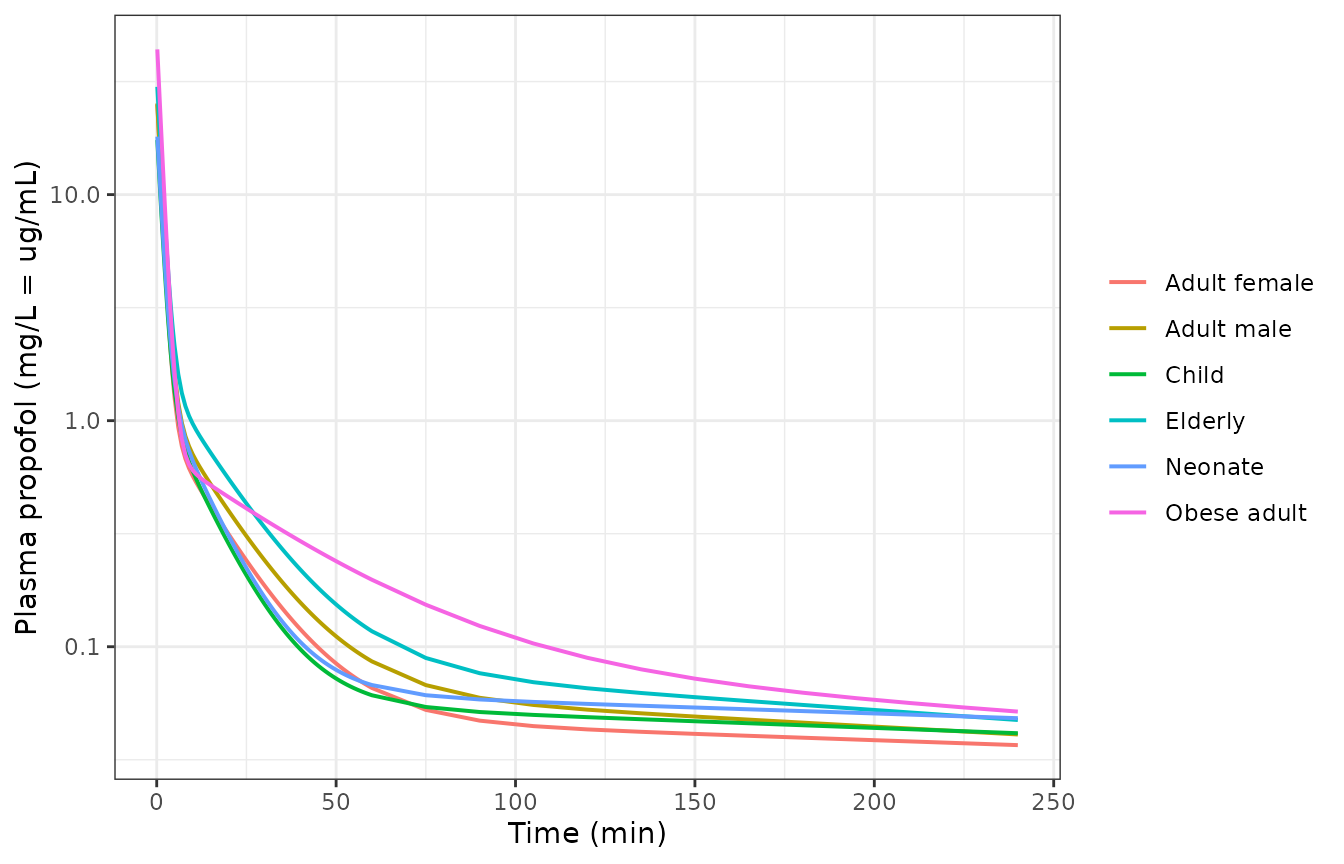
Simulated plasma propofol after a 2 mg/kg intravenous bolus in each representative subject. The paper’s own Figs. 4 and 5 are dataset-level diagnostics and cannot be redrawn without the Eleveld observations; see Errata.
Concentrations after induction are in the expected clinical range: the adult male reaches about 1.6 ug/mL at 5 min and about 0.7 ug/mL at 10 min after a 2 mg/kg bolus.
PKNCA validation
Non-compartmental analysis of the same simulation. Because the model
is linear and the profile is followed to 24 h, cl.obs and
vss.iv.obs recovered by NCA must reproduce the algebraic
Eq. 2 values exactly – this is an exact end-to-end gate on the ODE
implementation, not an approximate check.
conc_df <- sim |>
  dplyr::filter(!is.na(Cc)) |>
  dplyr::select(id, time, Cc, subject)

dose_df <- ev |>
  dplyr::filter(evid == 1) |>
  dplyr::select(id, time, amt, subject) |>
  dplyr::mutate(route = "intravascular", duration = 0)

conc_obj <- PKNCA::PKNCAconc(conc_df, Cc ~ time | subject + id,
                             concu = "mg/L", timeu = "s")
dose_obj <- PKNCA::PKNCAdose(dose_df, amt ~ time | subject + id,
                             route = "route", duration = "duration",
                             doseu = "mg")

intervals <- data.frame(
  start = 0, end = Inf,
  cmax = TRUE, tmax = TRUE, aucinf.obs = TRUE, half.life = TRUE,
  cl.obs = TRUE, vss.iv.obs = TRUE, mrt.iv.obs = TRUE, aucpext.obs = TRUE
)

nca <- PKNCA::pk.nca(PKNCA::PKNCAdata(conc_obj, dose_obj, intervals = intervals))
nca_res <- as.data.frame(nca) |>
  dplyr::filter(start == 0, end == Inf) |>
  dplyr::select(subject, id, PPTESTCD, PPORRES)
wide <- nca_res |>
  tidyr::pivot_wider(names_from = PPTESTCD, values_from = PPORRES) |>
  dplyr::left_join(pk, by = c("id", "subject")) |>
  dplyr::mutate(
    `CL NCA (L/min)` = cl.obs * 60,
    `CL Eq. 2 (L/min)` = CL,
    `Vss NCA (L)` = vss.iv.obs,
    `Vss Eq. 2 (L)` = Vss,
    `t1/2 (h)` = half.life / 3600,
    `AUC extrap (%)` = aucpext.obs
  )

wide |>
  dplyr::select(subject, `CL NCA (L/min)`, `CL Eq. 2 (L/min)`,
                `Vss NCA (L)`, `Vss Eq. 2 (L)`, `t1/2 (h)`, `AUC extrap (%)`) |>
  dplyr::rename("Subject" = subject) |>
  knitr::kable(digits = c(0, 3, 3, 1, 1, 2, 1),
caption = "NCA-recovered clearance and steady-state volume against the model's own Eq. 2 values.")| Subject | CL NCA (L/min) | CL Eq. 2 (L/min) | Vss NCA (L) | Vss Eq. 2 (L) | t1/2 (h) | AUC extrap (%) |
|---|---|---|---|---|---|---|
| Adult female | 1.578 | 1.578 | 561.7 | 562.7 | 9.17 | 7.2 |
| Adult male | 1.578 | 1.578 | 298.8 | 299.2 | 5.75 | 2.1 |
| Child | 0.487 | 0.488 | 186.7 | 187.1 | 8.51 | 7.3 |
| Elderly | 1.336 | 1.337 | 177.6 | 177.8 | 4.52 | 0.8 |
| Neonate | 0.073 | 0.073 | 34.0 | 34.0 | 9.55 | 9.8 |
| Obese adult | 1.939 | 1.940 | 266.3 | 266.7 | 4.87 | 1.0 |
stopifnot(
  "NCA clearance must equal kel * vc" =
    all(abs(wide$cl.obs / (wide$kel * wide$vc) - 1) < 0.02),
  "NCA Vss must equal V1 + V2 + V3" =
    all(abs(wide$vss.iv.obs / wide$Vss - 1) < 0.02)
)
Dose proportionality
The model is linear in dose, so doubling the bolus must double every exposure metric to within integration tolerance.
sim2 <- rxode2::rxSolve(mod, events = build_events(cohort, 2 * dose_mg_per_kg),
                        keep = c("subject", "dose_mg"), returnType = "data.frame",
                        rtol = 1e-10, atol = 1e-12)
#> Warning: multi-subject simulation without without 'omega'
ratio <- sim2$Cc[sim2$time > 0] / sim$Cc[sim$time > 0]
cat(sprintf("max |Cc(4 mg/kg) / Cc(2 mg/kg) - 2| = %.3g\n", max(abs(ratio - 2))))
#> max |Cc(4 mg/kg) / Cc(2 mg/kg) - 2| = 1.04e-09
stopifnot("Model must be exactly dose-linear" = max(abs(ratio - 2)) < 1e-6)
Shape of the learned covariate model
The covariate model is the paper’s actual result, so its shape is worth showing directly. Clearance, central volume and steady-state volume are evaluated over the covariate ranges of Table 1.
sweep <- function(varying, values, base) {
  g <- base[rep(1, length(values)), , drop = FALSE]
  g[[varying]] <- values
  g$id <- seq_along(values)
  g$subject <- as.character(g$id)
  p <- param_at_zero(g)
  p$x <- values
  p$SEXF <- g$SEXF
  dplyr::mutate(p,
    CL = kel * vc * 60,
    V1 = vc,
    Vss = vc + k12 / k21 * vc + k13 / k31 * vc
  )
}

grid <- dplyr::bind_rows(
  lapply(c(0, 1), function(sf) {
    base_age <- data.frame(AGE = 35, WT = 70, BMI = 24.2, SEXF = sf)
    base_wt <- data.frame(AGE = 35, WT = 70, BMI = 24.2, SEXF = sf)
    dplyr::bind_rows(
      dplyr::mutate(sweep("AGE", seq(0.05, 88, length.out = 120), base_age),
                    panel = "Age (years)"),
      dplyr::mutate(sweep("WT", seq(3, 160, length.out = 120), base_wt),
                    panel = "Weight (kg)")
    )
  })
)
#> Warning: multi-subject simulation without without 'omega'
#> Warning: multi-subject simulation without without 'omega'
#> Warning: multi-subject simulation without without 'omega'
#> Warning: multi-subject simulation without without 'omega'

grid |>
  tidyr::pivot_longer(c(CL, V1, Vss), names_to = "param", values_to = "value") |>
  dplyr::mutate(
    Sex = ifelse(SEXF == 1, "Female", "Male"),
    param = factor(param, c("CL", "V1", "Vss"),
                   c("CL (L/min)", "V1 (L)", "Vss (L)"))
  ) |>
  ggplot(aes(x, value, colour = Sex)) +
  geom_line(linewidth = 0.7) +
  facet_grid(param ~ panel, scales = "free") +
  labs(x = NULL, y = NULL, colour = NULL) +
  theme_bw()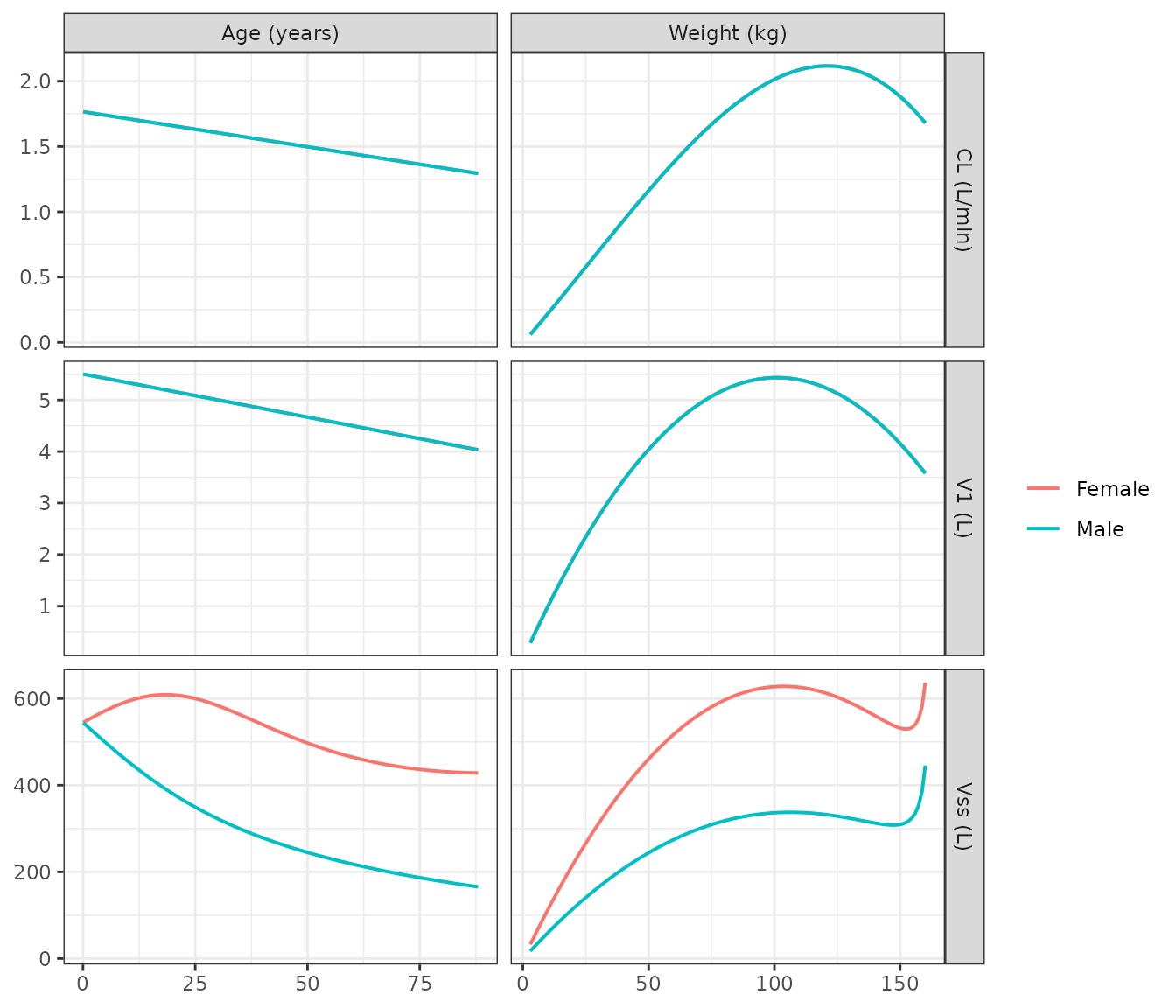
Learned covariate relationships (Eq. 10) over the Table 1 ranges. Left column: age sweep at 70 kg / BMI 24.2. Right column: weight sweep at age 35 y, BMI held at 24.2.
Clearance rises with weight and is essentially flat in age, V1 rises then saturates with weight (the negative squared-weight term in Eq. 10h), and the male/female split enters only through k13 and k31, which is why Vss separates by sex while CL and V1 do not.
Reproduction against the authors’ own deposited predictions
The paper’s Data availability statement points to a code and data
deposit (reference 27) that contains the Eleveld dataset, the authors’
trained network, and their per-observation predictions. Those files are
not redistributed with nlmixr2lib, so the check below is
not run at build time, but it was run during extraction and it is what
established the k12_norm correction documented under
Errata.
# git clone https://github.com/wahlquisty/learning-pharmacometric-covariate-structures
#
# Simulate every one of the 1,031 subjects on their recorded infusion history
# (eleveld_infusiondata.csv) with this model and compare against
# csv/predicted_observed_conc.csv, column
# "Predicted concentration symbolic regression ALE".
#
# Result obtained during extraction, over 15,395 of the 15,433 observations:
#
#   ratio (this model / authors' prediction)
#     5%     25%    50%    75%    95%
#   0.617   0.929  1.006  1.102  1.409
#
#   mean MdALE  this model 0.305 | authors' network 0.279 | Eleveld 0.325
#   paper Table 2           --   |                  0.279 |          0.325
#
# The authors' own numbers reproduce Table 2 exactly, confirming the row
# alignment and the MdALE implementation. This model, rebuilt from the
# three-significant-figure coefficients printed in Eq. 10, sits between the
# two: unbiased at the subject level (median ratio 1.006, per-subject median
# IQR 0.987-1.034) with residual within-subject profile scatter attributable
# to the printed rounding.
#
# Without the k12_norm factor the same comparison gives a median ratio of
# about 0.13 -- roughly sevenfold low.
Assumptions and deviations
Errata
Eq. 10b is published without its network-output normalisation
constant. Every expression in Eq. 10 is a symbolic-regression
network output multiplied by a per-parameter normalisation factor.
Dividing each printed expression by its factor (listed as
pkparams_normalization in
symbreg/checkresults/volumesclearances.jl of the
reference-27 deposit) should recover a raw network output of order one.
It does for five of the six parameters (0.26 to 0.85 at the reference
patient) but gives 19.2 for k12, which shows that Eq. 10b was printed
before scaling. Taken at face value, Eq. 10b gives k12 = 0.256
s^-1 for the reference patient, implying Q2 = 76 L/min and V2 = 828 L –
physiologically impossible, contradicting the paper’s own statement that
the volumes and clearances are comparable to Eleveld’s, and producing
plasma concentrations about sevenfold below the observed data.
Multiplying by the deposited k12 factor 0.013328808 gives k12 = 0.00341
s^-1, Q2 = 1.01 L/min, V2 = 11.0 L and Vss = 299 L, and reproduces the
authors’ own deposited per-observation predictions with a median ratio
of 1.006. The model file therefore carries
k12_norm <- fixed(0.013328808) with the provenance
recorded inline. This is a publication error in Eq. 10b, not a modelling
choice; no other equation is affected.
BMImax precision. The paper prints BMImax = 52.8 kg/m^2. The authors’ code uses the full-precision dataset maximum 52.84713965, which is what the model file uses. The difference is 0.09% on the normalised BMI.
No published figure can be redrawn. Figure 4 (predicted versus observed) and Figure 5 (MdALE boxplot) are both dataset-level diagnostics over the 1,031 Eleveld subjects. The dataset is openly available but is not redistributed with this package, so the figures are replaced here by the covariate-model shape plot and by the deposit reproduction described above.
Assumptions
-
No inter-individual variability. The model is
deterministic by construction: “the obtained covariate model is
deterministic in the sense that we do not obtain a distribution over
individual PK parameter values” (Discussion). No
etaterms are added. -
No residual-error model. None is reported, so
propSdisfixed(0)rather than invented. The paper’s accuracy statistic is MdALE = 0.279 (Table 2); it is a model-plus-residual accuracy measure, not a fitted residual standard deviation, and is deliberately not converted into one. -
Absolute values on every parameter. Eq. 8 defines
the final-layer base expression as g3(z3) = |z3|, so every network
output is non-negative. The paper prints the bars explicitly only on k12
(Eq. 10b) and k21 (Eq. 10e), where the argument changes sign over the
covariate range;
abs()is applied to all six outputs in the model file, which is faithful to Eq. 8 and a no-op wherever the argument is already positive. -
Sex encoded as a sign switch. Eqs. 10c/10d and
10f/10g differ only in the sign of their age-linear terms, so the four
printed expressions are encoded as two expressions with
sexsign = 1 - 2 * SEXF. This reproduces each printed form exactly. -
Peripheral compartments hold amounts. Eq. 1 is
written for xi = Ai / V1. Multiplying through by V1 gives the amount
form used in the model file, which is why
peripheral1andperipheral2carry true amounts and Eq. 2’s V2 = (k12/k21) V1 holds. - Representative subjects, not a virtual population. With no random effects, a simulated cohort adds nothing over a covariate grid, so six representative subjects spanning the Table 1 ranges are used.
-
Blood sampling site is documented but unused. It
was one of the five candidate covariates and was pruned automatically by
the algorithm, so it is recorded in
covariatesDataExcludedand is not a covariate of the model.
Reference
- Wahlquist Y, Sundell J, Soltesz K. Learning pharmacometric covariate model structures with symbolic regression networks. J Pharmacokinet Pharmacodyn. 2024;51(2):155-167. doi:10.1007/s10928-023-09887-3. PMCID: PMC11416364. Code and data deposit (cited as reference 27 of the paper): https://github.com/wahlquisty/learning-pharmacometric-covariate-structures
- Eleveld DJ, Colin P, Absalom AR, Struys MMRF. Pharmacokinetic-pharmacodynamic model for propofol for broad application in anaesthesia and sedation. Br J Anaesth. 2018;120(5):942-959. doi:10.1016/j.bja.2018.01.018