Caspofungin (Wang 2020)

Model and source

• Citation: Wang Q, Zhang Z, Liu D, Chen W, Cui G, Li P, Zhang X, Li M, Zhan Q, Wang C. Population pharmacokinetics of caspofungin among extracorporeal membrane oxygenation patients during the postoperative period of lung transplantation. Antimicrob Agents Chemother. 2020;64(11):e00687-20. doi:10.1128/AAC.00687-20. PMC7577146.
• Description: Two-compartment population PK model for intravenous caspofungin in adult lung transplant recipients during the early postoperative period, with and without veno-venous extracorporeal membrane oxygenation (ECMO) (Wang 2020). Operative time enters as a power covariate (centred at 5 h) on clearance and central volume, male sex as an additive shift in central volume, and the sequential organ failure assessment (SOFA) score as a power covariate on intercompartmental clearance. ECMO was screened and not retained. Exponential IIV on CL, Vc and Vp; additive residual error. NONMEM 7.2; 19 patients, 31 profiles, 271 samples.
• Article: https://doi.org/10.1128/AAC.00687-20
• Open-access full text: https://www.ncbi.nlm.nih.gov/pmc/articles/PMC7577146/

Wang 2020 studied caspofungin given as antifungal prophylaxis to adult lung transplant recipients in the first days after surgery. Twelve patients needed veno-venous ECMO; they were sampled on ECMO (the “ECMO group”) and again after weaning, as their own controls (“control group A”). Seven patients who never needed ECMO formed “control group B”. ECMO did not affect caspofungin PK. The final two-compartment model keeps three covariates: operative time on CL and Vc, male sex on Vc, and the SOFA score on Q.

Population

Nineteen patients from one centre in Beijing, China (October 2017 - March 2018) gave 271 plasma samples over 31 dosing-interval profiles (Wang 2020 Results and Table 1). The ECMO group had a median age of 65 years, weight 64 kg, 25% women and a median operative time of 4.0 h (IQR 3.5-5.0). Control group B had a median age of 59 years, weight 65 kg, 28.6% women and a median operative time of 5.5 h (5.0-5.8). The median SOFA score on the sampling day was 7 (6-10) in the ECMO group, 6 (5-9) after weaning, and 7 (6-8) in control group B (Table 2). Patients on renal replacement therapy were excluded. Every patient received 50 mg caspofungin intravenously every 24 h, with no loading dose. The first dose was given immediately after surgery.

Source trace

Model element	Value	Source location
Two-compartment model, IV infusion	–	Results, ‘Establishment of a pharmacokinetic model’
lcl (CL at T_SURG = 5 h)	0.21 L/h	Table 4
lvc (Vc, female, T_SURG = 5 h)	2.21 L	Table 4
lvp (Vp)	2.87 L	Table 4
lq (Q at SOFA = 7)	0.84 L/h	Table 4
e_t_surg_cl	1.30	Table 4, ‘Theta OPT on CL’
e_t_surg_vc	0.93	Table 4, ‘Theta OPT on VC’
e_sex_vc (additive, men)	0.62 L	Table 4, ‘Theta SEX on VC’
e_sofa_q	1.98	Table 4, ‘Theta SOFA on Q’
etalcl, etalvc, etalvp	0.04, 0.01, 0.23	Table 4, interindividual variability
addSd	0.73 mg/L	Table 4, residual error
CL = CL_TV (OPT/5)^theta exp(eta)	–	Results, first final-model equation
Vc = (Vc_TV + SEX theta) (OPT/5)^theta exp(eta)	–	Results, second final-model equation
Q = Q_TV (SOFA/7)^theta	–	Not printed. Power form from Methods, ‘Establishment of a covariate model’. Centring 7 = Table 2 median
Dose 50 mg q24h, sampling 0-24 h	–	Methods, ‘Drug regimen and the collection of pharmacokinetic data’

Virtual cohort

Each arm has 100 subjects. Operative time and SOFA are drawn log-normally, using each group’s median and an SD taken from its IQR. SOFA is rounded to an integer, and non-positive draws are redrawn. The simulated ECMO patients are reused as control group A, as in the study. Their SOFA score drops by one point after weaning (the Table 2 medians fall from 7 to 6). Their weaning occasion is the third dose, 48-72 h, which is the interval Table 3 reports for group A.

set.seed(2020)
rxode2::rxSetSeed(2020)
n_arm <- 100

draw_lnorm <- function(n, med, q25, q75, integer = FALSE, min_val = 0) {
  sdl <- log(q75 / q25) / 1.349
  out <- numeric(0)
  while (length(out) < n) {
    x <- exp(rnorm(n, log(med), sdl))
    if (integer) x <- round(x)
    out <- c(out, x[x > min_val])
  }
  out[seq_len(n)]
}

ecmo <- data.frame(
  id = seq_len(n_arm),
  group = "ECMO / control A",
  T_SURG = draw_lnorm(n_arm, 4.0, 3.5, 5.0),
  SOFA = draw_lnorm(n_arm, 7, 6, 10, integer = TRUE),
  SEXF = rbinom(n_arm, 1, 0.25)
)
ecmo$SOFA_A <- pmax(ecmo$SOFA - 1, 1)

ctlb <- data.frame(
  id = n_arm + seq_len(n_arm),
  group = "Control B",
  T_SURG = draw_lnorm(n_arm, 5.5, 5.0, 5.8),
  SOFA = draw_lnorm(n_arm, 7, 6, 8, integer = TRUE),
  SEXF = rbinom(n_arm, 1, 0.286)
)
ctlb$SOFA_A <- ctlb$SOFA

subj <- dplyr::bind_rows(ecmo, ctlb)
subj |>
  dplyr::group_by(group) |>
  dplyr::summarise(
    median_T_SURG = median(T_SURG), median_SOFA = median(SOFA),
    pct_female = 100 * mean(SEXF), .groups = "drop"
  ) |>
  knitr::kable(digits = 2, caption = "Virtual cohort covariates.")

Virtual cohort covariates.

group	median_T_SURG	median_SOFA	pct_female
Control B	5.40	7	25
ECMO / control A	4.13	7	24

The infusion duration is not stated in the paper. A 0.5 h infusion is used (see Assumptions and deviations).

inf_dur <- 0.5
dose_times <- c(0, 24, 48)
obs_times <- sort(unique(c(seq(0, 72, by = 0.25), 24 + c(0.5, 1, 2, 4, 8, 12, 24))))

make_events <- function(s) {
  dose <- data.frame(
    id = s$id, time = dose_times, evid = 1, amt = 50, rate = 50 / inf_dur,
    cmt = "central"
  )
  obs <- data.frame(id = s$id, time = obs_times, evid = 0, amt = 0, rate = 0, cmt = "central")
  ev <- rbind(dose, obs)
  ev$T_SURG <- s$T_SURG
  ev$SEXF <- s$SEXF
  # SOFA is time-varying for the ECMO patients: the weaning occasion (the
  # 48-72 h interval) uses the post-weaning score.
  ev$SOFA <- ifelse(ev$time >= 48, s$SOFA_A, s$SOFA)
  ev$group <- s$group
  ev[order(ev$time, -ev$evid), ]
}
events <- do.call(rbind, lapply(split(subj, subj$id), make_events))

Simulation

mod <- readModelDb("Wang_2020_caspofungin")
sim <- rxode2::rxSolve(mod, events, keep = c("group"), returnType = "data.frame")
#> ℹ parameter labels from comments will be replaced by 'label()'

Replicate Figure 2 (median concentration-time curves)

Figure 2 of Wang 2020 shows median observed concentrations over the 24-48 h interval (the 2nd dose) for the ECMO group and control group B, and over 48-72 h (the weaning occasion) for control group A. Below are the simulated medians and 5th-95th percentiles over the same intervals. The points are the observed Table 3 median Cmax and Cmin.

seg <- function(d, lo, lab) {
  d |>
    dplyr::filter(time >= lo, time <= lo + 24) |>
    dplyr::mutate(tad = time - lo, arm = lab)
}
fig_dat <- dplyr::bind_rows(
  seg(dplyr::filter(sim, group == "ECMO / control A"), 24, "ECMO group"),
  seg(dplyr::filter(sim, group == "ECMO / control A"), 48, "Control group A"),
  seg(dplyr::filter(sim, group == "Control B"), 24, "Control group B")
) |>
  dplyr::group_by(arm, tad) |>
  dplyr::summarise(
    med = median(Cc), lo = quantile(Cc, 0.05), hi = quantile(Cc, 0.95),
    .groups = "drop"
  )

obs_pts <- data.frame(
  arm = rep(c("ECMO group", "Control group A", "Control group B"), 2),
  tad = rep(c(0.5, 24), each = 3),
  conc = c(16.7, 18.3, 17.9, 3.5, 3.2, 3.5)
)

ggplot(fig_dat, aes(tad, med, colour = arm, fill = arm)) +
  geom_ribbon(aes(ymin = lo, ymax = hi), alpha = 0.15, colour = NA) +
  geom_line() +
  geom_point(data = obs_pts, aes(tad, conc), size = 2.5, shape = 21, colour = "black") +
  labs(
    x = "Time after start of infusion (h)", y = "Caspofungin (mg/L)",
    colour = NULL, fill = NULL,
    caption = "Replicates Figure 2 of Wang 2020. Points: observed median Cmax / Cmin (Table 3)."
  ) +
  theme_bw()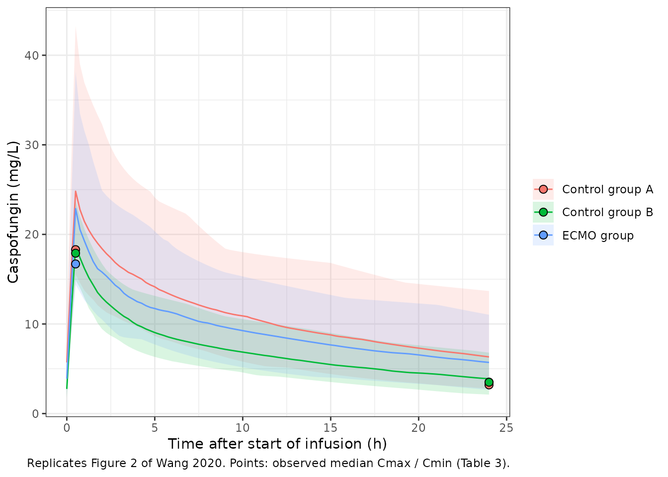

PKNCA validation

nca_intervals <- dplyr::bind_rows(
  data.frame(group = "ECMO / control A", arm = "ECMO group", start = 24, end = 48),
  data.frame(group = "ECMO / control A", arm = "Control group A", start = 48, end = 72),
  data.frame(group = "Control B", arm = "Control group B", start = 24, end = 48)
)

run_nca <- function(k) {
  iv <- nca_intervals[k, ]
  conc <- sim |>
    dplyr::filter(group == iv$group, !is.na(Cc)) |>
    dplyr::mutate(arm = iv$arm) |>
    dplyr::select(id, time, Cc, arm)
  dose <- events |>
    dplyr::filter(group == iv$group, evid == 1) |>
    dplyr::mutate(arm = iv$arm) |>
    dplyr::select(id, time, amt, arm)
  conc_obj <- PKNCA::PKNCAconc(conc, Cc ~ time | arm + id, concu = "mg/L", timeu = "h")
  dose_obj <- PKNCA::PKNCAdose(dose, amt ~ time | arm + id, doseu = "mg")
  intervals <- data.frame(
    start = iv$start, end = iv$end,
    cmax = TRUE, cmin = TRUE, auclast = TRUE
  )
  as.data.frame(PKNCA::pk.nca(PKNCA::PKNCAdata(conc_obj, dose_obj, intervals = intervals))$result)
}
nca_res <- dplyr::bind_rows(lapply(seq_len(nrow(nca_intervals)), run_nca))

nca_res |>
  dplyr::filter(PPTESTCD %in% c("cmax", "cmin", "auclast")) |>
  dplyr::group_by(arm, PPTESTCD) |>
  dplyr::summarise(
    median = median(PPORRES), q25 = quantile(PPORRES, 0.25),
    q75 = quantile(PPORRES, 0.75), .groups = "drop"
  ) |>
  dplyr::mutate(parameter = nlmixr2lib::ncaParamLabel(PPTESTCD)) |>
  dplyr::select(arm, parameter, median, q25, q75) |>
  dplyr::rename(
    "Group" = arm, "NCA parameter" = parameter, "Median" = median,
    "25th percentile" = q25, "75th percentile" = q75
  ) |>
  knitr::kable(digits = 2, caption = "Simulated NCA of the sampled interval (Cmax, Cmin in mg/L; AUC in mg.h/L).")

Simulated NCA of the sampled interval (Cmax, Cmin in mg/L; AUC in mg.h/L).

Group	NCA parameter	Median	25th percentile	75th percentile
Control group A	AUClast	265.09	217.89	342.76
Control group A	Cmax	24.82	21.47	31.88
Control group A	Cmin	5.71	4.34	7.80
Control group B	AUClast	172.00	149.14	203.09
Control group B	Cmax	18.69	17.18	20.38
Control group B	Cmin	2.75	2.31	3.50
ECMO group	AUClast	232.64	192.84	287.69
ECMO group	Cmax	22.88	19.65	29.21
ECMO group	Cmin	3.88	3.06	5.01

Comparison against the published NCA (Table 3)

published <- data.frame(
  arm = c("ECMO group", "Control group A", "Control group B"),
  cmax = c(16.7, 18.3, 17.9),
  cmin = c(3.5, 3.2, 3.5),
  auclast = c(163.06, 147.11, 156.2)
)
cmp <- nlmixr2lib::ncaComparisonTable(
  simulated = nca_res,
  reference = published,
  by = "arm",
  params = c("cmax", "cmin", "auclast"),
  units = c(cmax = "mg/L", cmin = "mg/L", auclast = "mg*h/L"),
  tolerance_pct = 20
)
knitr::kable(cmp, caption = "Simulated vs published medians (Wang 2020 Table 3). * differs by >20%.")

Simulated vs published medians (Wang 2020 Table 3). * differs by >20%.

NCA parameter	arm	Reference	Simulated	% diff
Cmax (mg/L)	ECMO group	16.7	22.9	+37.0%*
Cmax (mg/L)	Control group A	18.3	24.8	+35.6%*
Cmax (mg/L)	Control group B	17.9	18.7	+4.4%
Cmin (mg/L)	ECMO group	3.5	3.88	+10.9%
Cmin (mg/L)	Control group A	3.2	5.71	+78.4%*
Cmin (mg/L)	Control group B	3.5	2.75	-21.4%*
AUClast (mg*h/L)	ECMO group	163	233	+42.7%*
AUClast (mg*h/L)	Control group A	147	265	+80.2%*
AUClast (mg*h/L)	Control group B	156	172	+10.1%

attr(cmp, "footnote")
#> [1] "* differs from reference by more than ±20%."

The model reproduces control group B, whose median operative time (5.5 h) is close to the 5 h centring value: Cmax and AUC are within about 10%. It overpredicts the two groups with short operations (median 4.0 h). Their Cmax is about 35% high, and their AUC is about 45% high on ECMO and 80% high after weaning. Control group A also shows some accumulation in the model, because its interval is the third dose. The observed group A AUC is, if anything, lower than the ECMO group’s. The final-model estimates in Table 4 cause this, not the simulation. Two things show it:

• Table 3 reports individual clearances with medians of 0.27-0.31 L/h in every group. The Table 4 typical CL is 0.21 L/h at 5 h of operative time, and only 0.16 L/h at the ECMO group’s median of 4.0 h. Likewise, Table 3 reports individual Vc medians of 2.9-3.2 L, but the model gives a typical 2.30 L for a man at 4.0 h. With IIV variances of only 0.04 on CL and 0.01 on Vc, the model cannot give the Table 3 values.
• The Table 4 point estimates for CL (0.21), Vc (2.21) and Q (0.84) all lie outside their own bootstrap 95% CIs (0.23-0.29, 2.45-2.89 and 0.86-1.28). The Results say that they lie inside.

The comparison below uses typical values: the zero-IIV solve at each group’s median covariates, for a man. It sets the published estimates beside the bootstrap medians from the same table. The bootstrap medians reduce the AUC overprediction, which confirms that the Table 4 estimates cause the gap. The model file keeps the published final estimates. The bootstrap medians are only a diagnostic here and are never used in the model.

typ_subj <- data.frame(
  arm = c("ECMO group", "Control group A", "Control group B"),
  T_SURG = c(4.0, 4.0, 5.5), SOFA = c(7, 6, 7), SEXF = 0,
  start = c(24, 48, 24)
)

typ_auc <- function(m) {
  out <- lapply(seq_len(nrow(typ_subj)), function(k) {
    s <- typ_subj[k, ]
    ev <- rxode2::et(amt = 50, rate = 50 / inf_dur, ii = 24, addl = 2, cmt = "central") |>
      rxode2::et(seq(0, 72, by = 0.05))
    ev <- as.data.frame(ev)
    ev$T_SURG <- s$T_SURG
    ev$SOFA <- s$SOFA
    ev$SEXF <- s$SEXF
    r <- rxode2::rxSolve(rxode2::zeroRe(m), ev, returnType = "data.frame")
    r <- r[r$time >= s$start & r$time <= s$start + 24, ]
    data.frame(
      arm = s$arm,
      auc = sum(diff(r$time) * (head(r$Cc, -1) + tail(r$Cc, -1)) / 2),
      cmin = r$Cc[nrow(r)]
    )
  })
  do.call(rbind, out)
}

boot_mod <- mod |>
  rxode2::ini(lcl = log(0.26), lvc = log(2.61), lvp = log(2.98), lq = log(1.00),
              e_t_surg_cl = 1.31, e_sex_vc = 0.64, e_t_surg_vc = 0.87, e_sofa_q = 2.04)
#> ℹ parameter labels from comments will be replaced by 'label()'
#> ℹ change initial estimate of `lcl` to `-1.34707364796661`
#> ℹ change initial estimate of `lvc` to `0.959350221334602`
#> ℹ change initial estimate of `lvp` to `1.09192330051731`
#> ℹ change initial estimate of `lq` to `0`
#> ℹ change initial estimate of `e_t_surg_cl` to `1.31`
#> ℹ change initial estimate of `e_sex_vc` to `0.64`
#> ℹ change initial estimate of `e_t_surg_vc` to `0.87`
#> ℹ change initial estimate of `e_sofa_q` to `2.04`

tv <- typ_auc(mod) |>
  dplyr::rename(auc_final = auc, cmin_final = cmin) |>
  dplyr::left_join(
    typ_auc(boot_mod) |> dplyr::rename(auc_boot = auc, cmin_boot = cmin),
    by = "arm"
  ) |>
  dplyr::left_join(published[, c("arm", "auclast")], by = "arm") |>
  dplyr::mutate(
    ratio_final = auc_final / auclast,
    ratio_boot = auc_boot / auclast
  )
#> ℹ parameter labels from comments will be replaced by 'label()'
#> ℹ omega/sigma items treated as zero: 'etalcl', 'etalvc', 'etalvp'
#> ℹ parameter labels from comments will be replaced by 'label()'
#> ℹ omega/sigma items treated as zero: 'etalcl', 'etalvc', 'etalvp'
#> ℹ parameter labels from comments will be replaced by 'label()'
#> ℹ omega/sigma items treated as zero: 'etalcl', 'etalvc', 'etalvp'
#> ℹ omega/sigma items treated as zero: 'etalcl', 'etalvc', 'etalvp'
#> ℹ omega/sigma items treated as zero: 'etalcl', 'etalvc', 'etalvp'
#> ℹ omega/sigma items treated as zero: 'etalcl', 'etalvc', 'etalvp'

tv |>
  dplyr::select(arm, auclast, auc_final, ratio_final, auc_boot, ratio_boot) |>
  dplyr::rename(
    "Group" = arm, "Observed median AUC (Table 3)" = auclast,
    "Typical AUC, Table 4 estimates" = auc_final, "Ratio (estimates)" = ratio_final,
    "Typical AUC, bootstrap medians" = auc_boot, "Ratio (bootstrap)" = ratio_boot
  ) |>
  knitr::kable(digits = 2, caption = "Typical-value AUC over the sampled interval (mg.h/L), male, group-median covariates.")

Typical-value AUC over the sampled interval (mg.h/L), male, group-median covariates.

Group	Observed median AUC (Table 3)	Typical AUC, Table 4 estimates	Ratio (estimates)	Typical AUC, bootstrap medians	Ratio (bootstrap)
ECMO group	163.06	242.06	1.48	206.03	1.26
Control group A	147.11	279.18	1.90	233.35	1.59
Control group B	156.20	177.32	1.14	148.84	0.95

# Deterministic (no random draws), so tight bounds are correct. They pin the
# documented overprediction of the published estimates, and the bootstrap
# medians' smaller gap.
ratio <- setNames(tv$ratio_final, tv$arm)
stopifnot(
  abs(ratio[["ECMO group"]] - 1.48) < 0.03,
  abs(ratio[["Control group A"]] - 1.90) < 0.03,
  abs(ratio[["Control group B"]] - 1.14) < 0.03,
  all(tv$ratio_boot < tv$ratio_final)
)

Structural checks

At steady state, the AUC over one dosing interval equals Dose / CL. The check uses the typical-value model and runs the PKNCA AUC over the 20th interval.

ss_ev <- rxode2::et(amt = 50, rate = 50 / inf_dur, ii = 24, addl = 19, cmt = "central") |>
  rxode2::et(seq(0, 480, by = 0.05)) |>
  as.data.frame()
ss_ev$T_SURG <- 5
ss_ev$SOFA <- 7
ss_ev$SEXF <- 0
ss_ev$id <- 1L
ss <- rxode2::rxSolve(rxode2::zeroRe(mod), ss_ev, returnType = "data.frame")
#> ℹ parameter labels from comments will be replaced by 'label()'
#> ℹ omega/sigma items treated as zero: 'etalcl', 'etalvc', 'etalvp'
ss$id <- 1L

conc_ss <- PKNCA::PKNCAconc(ss[, c("id", "time", "Cc")], Cc ~ time | id)
dose_ss <- PKNCA::PKNCAdose(ss_ev[ss_ev$evid == 1, c("id", "time", "amt")], amt ~ time | id)
ss_nca <- as.data.frame(PKNCA::pk.nca(PKNCA::PKNCAdata(
  conc_ss, dose_ss,
  intervals = data.frame(start = 456, end = 480, auclast = TRUE)
))$result)
auc_tau <- ss_nca$PPORRES[ss_nca$PPTESTCD == "auclast"]
c(auc_tau = auc_tau, dose_over_cl = 50 / 0.21)
#>      auc_tau dose_over_cl 
#>     238.0948     238.0952
stopifnot(abs(auc_tau * 0.21 / 50 - 1) < 0.005)

The covariate equations are checked against hand calculation.

chk <- ss[1, c("cl", "vc", "vp", "q")]
stopifnot(
  abs(chk$cl - 0.21) < 1e-8, abs(chk$vc - (2.21 + 0.62)) < 1e-8,
  abs(chk$vp - 2.87) < 1e-8, abs(chk$q - 0.84) < 1e-8
)
one <- function(T_SURG, SOFA, SEXF) {
  e <- data.frame(id = 1L, time = c(0, 1), evid = c(1, 0), amt = c(50, 0),
                  cmt = "central", T_SURG = T_SURG, SOFA = SOFA, SEXF = SEXF)
  r <- rxode2::rxSolve(rxode2::zeroRe(mod), e, returnType = "data.frame")
  r[1, c("cl", "vc", "q")]
}
m4 <- one(4, 10, 0)
#> ℹ parameter labels from comments will be replaced by 'label()'
#> ℹ omega/sigma items treated as zero: 'etalcl', 'etalvc', 'etalvp'
stopifnot(
  abs(m4$cl - 0.21 * (4 / 5)^1.30) < 1e-8,
  abs(m4$vc - (2.21 + 0.62) * (4 / 5)^0.93) < 1e-8,
  abs(m4$q - 0.84 * (10 / 7)^1.98) < 1e-8
)
f4 <- one(4, 10, 1)
#> ℹ parameter labels from comments will be replaced by 'label()'
#> ℹ omega/sigma items treated as zero: 'etalcl', 'etalvc', 'etalvp'
stopifnot(abs(f4$vc - 2.21 * (4 / 5)^0.93) < 1e-8)

Assumptions and deviations

• The Q equation is not printed. The Results print only the CL and Vc equations, but Table 4 has an estimate for “Theta SOFA on Q”. The Q term uses the paper’s general continuous-covariate form, (Cov / Cov median)^theta (Methods), centred at a SOFA of 7. That is the median of both the ECMO group and control group B (Table 2). The weaning occasions had a median of 6, so the median over all 31 occasions may be 6 or 7. A centring of 6 would raise typical Q by (7/6)^1.98, or 36%, at any given SOFA score.
• Sex coding. In the printed Vc equation, sex is an additive shift, (Vc_TV + SEX x 0.62) L. The Methods describe categorical covariates as exp(theta) multipliers, but where the text and a printed equation disagree, the equation is followed. The abstract and Discussion say that male sex increases the distribution volume, so SEX = 1 is taken to mean male. It enters as (1 - SEXF). The 2.21 L typical value is therefore the female value.
• Residual error. The Methods describe a combined proportional-plus-additive error. The Results text calls it “proportional”, and Table 4 lists a single “Additive (mg/liter)” term of 0.73. With the units in mg/L, this term is encoded as an additive SD. No proportional value is reported, so none is invented.
• IIV scale. The Table 4 interindividual-variability values (0.04, 0.01, 0.23) are read as omega^2 (variances of eta). These are the values NONMEM estimates, and none of them is labelled as a CV%.
• Infusion duration. The paper does not state the infusion duration. In Figure 2 the median concentration is higher at 0.5 h than at 1 h. The infusion therefore ended by 0.5 h, and a 0.5 h infusion is used. The licensed ~1 h infusion would give a lower 0.5 h concentration than the one observed.
• The published estimates do not reproduce the published exposures. See the NCA comparison. The final-model estimates are extracted as published and have not been adjusted. The bootstrap medians are shown only as a diagnostic.
• Cohort. The covariate distributions come from group medians and IQRs. The weaning-occasion SOFA is the on-ECMO value minus one point. Figure 4 (the VPC) cannot be replicated without the observed data.