Pediatric sulbactam-durlobactam dose selection (Larson 2026)

Model and source

• Citation: Larson KB, O’Donnell J, Tanudra A, Cammarata AP, Rubino CM. P-444. Population Pharmacokinetics (PPK) Analysis of Sulbactam-Durlobactam (SUD) to Support Dose Selection for Evaluation in a Clinical Trial in Pediatric Patients with Acinetobacter Baumannii-Calcoaceticus Complex (ABC) Infections. Open Forum Infect Dis. 2026;13(Suppl 1):S405. doi:10.1093/ofid/ofaf695.659. PMCID: PMC12792777. The model specification is taken from the corresponding IDWeek 2025 poster, which carries a different author order: Cammarata A, Larson KB, Tanudra A, O’Donnell JP, Bhavnani SM, Rubino CM. ‘Population pharmacokinetics analysis of sulbactam-durlobactam to support the dose selection for evaluation in a clinical trial in pediatric patients with Acinetobacter baumannii-calcoaceticus complex infections.’ Poster P-444, IDWeek 2025, Atlanta, GA. All structural, covariate, IIV and residual-error values are inherited unchanged from the adult parent model: Cammarata AP, Safir MC, Trang M, Larson KB, O’Donnell JP, Bhavnani SM, Rubino CM. Population pharmacokinetic analyses for sulbactam-durlobactam using Phase 1, 2, and 3 data. Antimicrob Agents Chemother. 2025;69(1):e00485-24. doi:10.1128/aac.00485-24; see modellib(‘Cammarata_2024_sulbactam_durlobactam’).

• Abstract: https://doi.org/10.1093/ofid/ofaf695.659 (Open Forum Infect Dis 2026;13(Suppl 1):S405; PMCID PMC12792777, open access)

• Poster: IST_Poster-PPK_SUD_Pediatric_Oct2025_FINAL.pdf, presented as poster P-444 at IDWeek 2025 (Atlanta, GA) and posted publicly by Innoviva Specialty Therapeutics. The poster, not the abstract, is the source of the model specification — the abstract contains no parameter values, no equations and no covariate structure.

Note the author order differs between the two records. The indexed abstract is Larson, O’Donnell, Tanudra, Cammarata, Rubino; the poster is Cammarata, Larson, Tanudra, O’Donnell, Bhavnani, Rubino. The packaged files are named for the abstract’s first author, which is the citable, PubMed-indexed record.

Sulbactam-durlobactam (XACDURO) is approved in the United States for hospital-acquired and ventilator-associated bacterial pneumonia caused by susceptible Acinetobacter baumannii-calcoaceticus complex in patients aged 18 years and older. No pediatric clinical trial data existed when this analysis was done, so the pediatric dosing regimens for the Phase 1b trial CS2514-2023-002 (NCT06801223) were selected by scaling the published adult population PK model.

Two models, one change

The poster explored two approaches, and both are packaged:

mod_allo <- readModelDb("Larson_2026_sulbactam_durlobactam_pediatric_allometry")
mod_crcl <- readModelDb("Larson_2026_sulbactam_durlobactam_pediatric_allometry_crcl")
mod_adult <- readModelDb("Cammarata_2024_sulbactam_durlobactam")

Adult with Allometry (..._pediatric_allometry) is the model that guided dose selection. Poster Methods:

The first approach utilized the full covariate model from adults with the only change being the use of allometric scaling with fixed exponents of 0.75 for clearance and 1.0 for volume of distribution

with a Figure 1 note adding

WTKG effects added to Q and Vp for both drugs to account for likely changes in these parameters in children

Allometry + CL_CR (..._pediatric_allometry_crcl) is the alternative:

The second approach removed all covariate relationships from the Adult Allometry model except for body weight (on all parameters) and renal function (on renal clearance only)

The parent adult model is Cammarata_2024_sulbactam_durlobactam — a four-compartment (two per drug) linear model in which total clearance of each drug is the sum of a renal arm scaled by baseline BSA-normalized creatinine clearance and a non-renal arm:

$$\mathrm{CL_R} = \mathrm{CL}\cdot \mathrm{FE}\cdot\left(\frac{\mathrm{CLcr}}{100}\right)^{\theta_{\mathrm{CLcr}}}, \qquad \mathrm{CL_{NR}} = \mathrm{CL}\cdot(1-\mathrm{FE})$$

The pediatric adaptation replaces the adult body-weight terms:

$$\mathrm{CL_T} = (\mathrm{CL_R}+\mathrm{CL_{NR}}) \cdot\left(\frac{\mathrm{WT}}{75}\right)^{0.75}\cdots, \qquad \mathrm{V_c},\mathrm{V_p} \propto \left(\frac{\mathrm{WT}}{75}\right)^{1.0}, \qquad \mathrm{Q} \propto \left(\frac{\mathrm{WT}}{75}\right)^{0.75}$$

Population

This is a simulation population, not an estimation data set. Every parameter value was estimated in adults (373 subjects, 5,188 plasma concentrations, six Phase 1 + one Phase 2 + one Phase 3 study; Cammarata 2024) and re-used unchanged. The poster generated 8,000 hypothetical pediatric patients, 1,000 per cohort, spanning birth (28 weeks of gestation) to < 18 years, with age- and sex-appropriate body size from CDC growth charts and normal renal function.

str(readModelDb("Larson_2026_sulbactam_durlobactam_pediatric_allometry")()$population,
    max.level = 1)
#> List of 9
#>  $ species       : chr "human"
#>  $ n_subjects    : int 8000
#>  $ n_studies     : int 0
#>  $ age_range     : chr "birth (28 weeks of gestation) to < 18 years"
#>  $ weight_range  : chr "not reported; CDC growth-chart body size by age and sex"
#>  $ disease_state : chr "Simulated pediatric patients with Acinetobacter baumannii-calcoaceticus complex infection. This is a SIMULATION"| __truncated__
#>  $ dose_range    : chr "Simulations supporting the Phase 1b regimens of poster P-444 Table 2: 25 mg/kg sulbactam with 25 mg/kg durlobac"| __truncated__
#>  $ renal_function: chr "Normal renal function was assumed throughout. Poster P-444 Methods: the simulated dataset incorporated 'age- an"| __truncated__
#>  $ notes         : chr "8,000 hypothetical pediatric patients, 1,000 per cohort across the eight age / maturity cohorts of poster P-444"| __truncated__

Source trace

Almost every ini() value in these two models is inherited unchanged from the adult parent model; the poster re-used the adult estimates and changed only the body-size terms. The table below therefore separates the two provenances.

Equation / parameter	Value	Source location
e_wt_cl, e_wt_cl_sbt	0.75 (FIXED)	Poster P-444 Methods, first bullet (“fixed exponents of 0.75 for clearance”)
e_wt_vc, e_wt_vc_sbt	1.0 (FIXED)	Poster P-444 Methods, first bullet (“1.0 for volume of distribution”)
e_wt_q, e_wt_q_sbt	0.75 (FIXED)	Poster P-444 Figure 1 notes (“WTKG effects added to Q and Vp for both drugs”) + Methods bullet (0.75 for clearance)
e_wt_vp, e_wt_vp_sbt	1.0 (FIXED)	Poster P-444 Figure 1 notes + Methods bullet (1.0 for volume)
Covariate set retained (model 1)	full adult model	Poster P-444 Methods, first bullet (“the full covariate model from adults”)
Covariate set retained (model 2)	WT + CLcr on renal CL only	Poster P-444 Methods, second bullet
Infection type = bacteremia in the simulations	n/a	Poster P-444 Figure 1 notes (“Infection type was set to ‘Bacteremia’”)
Region = non-East-Asian in the simulations	n/a	Poster P-444 Figure 1 notes (“East Asian flag was set to ‘not East Asian’”)
CLcr units mL/min/1.73 m^2	n/a	Poster P-444 Figure 1 notes (“CL CR represents GFR normalized to BSA”)
Pediatric dosing regimens	see below	Poster P-444 Table 2
Adult reference exposures	see below	Poster P-444 Table 1
PK/PD targets	50% fT>MIC (SUL); fAUC/MIC 10 (DUR)	Poster P-444 Methods, PK/PD drivers
lcl, lvc, lq, lvp (durlobactam)	9.33 L/h, 12.5 L, 4.43 L/h, 5.83 L	Inherited: Cammarata 2024 Table 1, Durlobactam
lcl_sbt, lvc_sbt, lq_sbt, lvp_sbt	13.5 L/h, 12 L, 7.88 L/h, 6.99 L	Inherited: Cammarata 2024 Table 1, Sulbactam
f_renal, f_renal_sbt	0.479 (FIXED)	Inherited: Cammarata 2024 Table 1, FE (%)
e_crcl_cl_renal, e_crcl_cl_renal_sbt	0.875, 1.14	Inherited: Cammarata 2024 Table 1, CL R, CLcr power
Infection / region / severe-renal-impairment shifts	see model file	Inherited: Cammarata 2024 Table 1
e_hemodial_active_cl(_sbt)	log(6.24), log(8.19)	Inherited: Cammarata 2024 Table S4
lrelf, lrelf_sbt	log(0.372), log(0.533)	Inherited: Cammarata 2024 Table S6
All IIV and residual-error terms	see model file	Inherited: Cammarata 2024 Tables 1 and S4/S6
Reference weight 75 kg	n/a	Inherited: Cammarata 2024 Results reference subject; the poster does not restate it (see Errata)
Reference CLcr 100 mL/min/1.73 m^2	n/a	Inherited: Cammarata 2024 Results reference subject

Mechanical check that the inheritance is exact

The claim “the only change is the allometric scaling” is machine-checkable: compare every ini() estimate against the adult parent model.

ui <- function(m) rxode2::rxode(m)

tv <- function(u) {
  d <- u$iniDf
  d <- d[is.na(d$neta1), ]
  stats::setNames(d$est, d$name)
}

a <- tv(ui(mod_adult))
b <- tv(ui(mod_allo))
d2 <- tv(ui(mod_crcl))

shared     <- intersect(names(a), names(b))
differing  <- shared[abs(a[shared] - b[shared]) > 1e-12]
added      <- setdiff(names(b), names(a))
dropped_1  <- setdiff(names(a), names(b))

tibble::tibble(
  Parameter  = differing,
  Adult      = unname(a[differing]),
  Pediatric  = unname(b[differing])
) |>
  dplyr::rename("Adult (Cammarata 2024)" = Adult,
                "Pediatric (allometry)"  = Pediatric) |>
  knitr::kable(
    caption = paste(
      "Every ini() parameter that differs between the adult parent model and",
      "the 'Adult with Allometry' pediatric model. These four rows are the",
      "entire change the poster describes."
    )
  )

Every ini() parameter that differs between the adult parent model and the ‘Adult with Allometry’ pediatric model. These four rows are the entire change the poster describes.

Parameter	Adult (Cammarata 2024)	Pediatric (allometry)
e_wt_cl	0.646	0.75
e_wt_vc	0.521	1.00
e_wt_cl_sbt	1.010	0.75
e_wt_vc_sbt	0.831	1.00

# Structural gate. The poster says the ONLY change is the allometric scaling,
# so exactly the four body-weight exponents may differ, the four new Q / Vp
# exponents may be added, and NOTHING may be dropped.
stopifnot(
  setequal(differing, c("e_wt_cl", "e_wt_vc", "e_wt_cl_sbt", "e_wt_vc_sbt")),
  setequal(added, c("e_wt_q", "e_wt_vp", "e_wt_q_sbt", "e_wt_vp_sbt")),
  length(dropped_1) == 0L,
  # The eight allometric exponents must be FIXED, not estimated.
  all(ui(mod_allo)$iniDf$fix[grepl("^e_wt_", ui(mod_allo)$iniDf$name)]),
  all(ui(mod_crcl)$iniDf$fix[grepl("^e_wt_", ui(mod_crcl)$iniDf$name)]),
  # ... and take exactly the poster's two values.
  all(b[c("e_wt_cl", "e_wt_cl_sbt", "e_wt_q", "e_wt_q_sbt")] == 0.75),
  all(b[c("e_wt_vc", "e_wt_vc_sbt", "e_wt_vp", "e_wt_vp_sbt")] == 1.0)
)

# The second approach keeps the same allometry but drops every covariate
# relationship except CLcr on the renal arm.
shared2 <- intersect(names(a), names(d2))
stopifnot(
  setequal(shared2[abs(a[shared2] - d2[shared2]) > 1e-12],
           c("e_wt_cl", "e_wt_vc", "e_wt_cl_sbt", "e_wt_vc_sbt")),
  # CLcr on the renal arm survives ...
  all(c("e_crcl_cl_renal", "e_crcl_cl_renal_sbt") %in% names(d2)),
  # ... and every infection-type, region, severe-renal-impairment and
  # hemodialysis term is gone.
  !any(grepl("^e_(habp|vabp|cuti|bacteremia|ap|region|renalimp|hemodial)",
             names(d2)))
)

# Both models must keep explicit ODEs. A cl / vc pair can make rxode2 silently
# auto-solve a model and discard the d/dt() block; linCmt() would be non-empty.
stopifnot(length(ui(mod_allo)$linCmt) == 0L,
          length(ui(mod_crcl)$linCmt) == 0L)

Structural checks

The pediatric model reduces exactly to the adult model at 75 kg

Every allometric factor is (WT / 75)^k, so at WT = 75 kg all four factors are exactly 1 and the “Adult with Allometry” model must return the adult model’s own typical-value parameters. This is an exact identity, not an approximation.

#' Build a dose + observation event table for the four-compartment SUD model.
#'
#' Doses are 3-hour IV infusions of `dose_mg` of EACH drug into its own central
#' compartment. Observations sit on the durlobactam ODE state `central`;
#' rxode2 returns every algebraic observable (Cc, Cc_sbt, Celf, Celf_sbt) as a
#' column at those rows.
make_events <- function(subj, dose_mg, tau, tmax, by = 0.25) {
  doses <- subj |>
    tidyr::crossing(time = seq(0, tmax - tau, by = tau),
                    cmt = c("central", "central_sbt")) |>
    dplyr::mutate(evid = 1L, amt = dose_mg, rate = dose_mg / 3,
                  dvid = NA_integer_)
  obs <- subj |>
    tidyr::crossing(time = seq(0, tmax, by = by)) |>
    dplyr::mutate(evid = 0L, amt = NA_real_, rate = NA_real_,
                  cmt = "central", dvid = 1L)
  dplyr::bind_rows(doses, obs) |> dplyr::arrange(id, time, dplyr::desc(evid))
}

#' Solve at typical values (no IIV, no residual error).
solve_typical <- function(mod, events, keep) {
  rxode2::rxSolve(
    rxode2::zeroRe(mod), events = events, keep = keep,
    omega = NA, sigma = NA,
    # rxode2's automatic ODE -> linCmt() conversion mis-maps the outputs of
    # this four-compartment two-analyte model; disable it.
    useLinCmt = FALSE
  ) |> as.data.frame()
}

trapz <- function(x, y) sum(diff(x) * (utils::head(y, -1) + utils::tail(y, -1)) / 2)

# The poster's simulation settings, applied to every cohort:
#   infection type = bacteremia, region = not East Asian, normal renal function.
POSTER_COVS <- list(
  CRCL                = 100,   # "normal renal function"; the model's own reference
  RENALIMP_SEV        = 0,
  REGION_EASTASIA     = 0,
  DIS_HABP            = 0, DIS_VABP = 0, DIS_CUTI = 0,
  DIS_BACTEREMIA      = 1, DIS_AP   = 0,
  RRT_HEMODIAL_ACTIVE = 0,
  STUDY_SULDUR_PHASE2 = 0, STUDY_SULDUR_PHASE3 = 1
)

ref_subj <- tibble::as_tibble(c(list(id = 1L, WT = 75), POSTER_COVS))

ref_ev  <- make_events(ref_subj, dose_mg = 1000, tau = 6, tmax = 12)
sim_ped <- solve_typical(mod_allo,  ref_ev, keep = "WT")
sim_ad  <- solve_typical(mod_adult, ref_ev, keep = "WT")

pars <- c("cl", "vc", "q", "vp", "cl_sbt", "vc_sbt", "q_sbt", "vp_sbt")
cmp_75 <- tibble::tibble(
  Parameter  = pars,
  Adult      = vapply(pars, \(p) sim_ad[[p]][1],  numeric(1)),
  Pediatric  = vapply(pars, \(p) sim_ped[[p]][1], numeric(1))
) |>
  dplyr::mutate(`Ratio` = Pediatric / Adult)

cmp_75 |>
  dplyr::rename("Adult model at 75 kg" = Adult,
                "Pediatric allometry model at 75 kg" = Pediatric) |>
  knitr::kable(
    digits  = 6,
    caption = paste(
      "At the 75 kg reference weight every allometric factor is exactly 1, so",
      "the pediatric model must return the adult model's typical-value",
      "clearances (L/h) and volumes (L) identically."
    )
  )

At the 75 kg reference weight every allometric factor is exactly 1, so the pediatric model must return the adult model’s typical-value clearances (L/h) and volumes (L) identically.

Parameter	Adult model at 75 kg	Pediatric allometry model at 75 kg	Ratio
cl	9.330	9.330	1
vc	54.000	54.000	1
q	4.430	4.430	1
vp	5.830	5.830	1
cl_sbt	7.506	7.506	1
vc_sbt	34.200	34.200	1
q_sbt	7.880	7.880	1
vp_sbt	6.990	6.990	1

# Exact identity: this is deterministic algebra, not a simulated statistic, so
# the bound is machine precision rather than a tolerance.
stopifnot(max(abs(cmp_75$Ratio - 1)) < 1e-10)

The allometric exponents are exactly 0.75 and 1.0

Solving at two weights recovers the exponents by $\log(P_2/P_1)\,/\,\log(\mathrm{WT}_2/\mathrm{WT}_1)$. With every other covariate held fixed this must return 0.75 for the two clearances and 1.0 for the two volumes, for both drugs.

w_subj <- tibble::as_tibble(c(list(id = 1:2, WT = c(10, 60)), POSTER_COVS))
w_sim  <- solve_typical(mod_allo, make_events(w_subj, 500, 6, 6), keep = "WT")

first_by_id <- w_sim |> dplyr::group_by(id) |> dplyr::slice(1) |> dplyr::ungroup()

exps <- tibble::tibble(
  Parameter = pars,
  Recovered = vapply(
    pars,
    \(p) log(first_by_id[[p]][2] / first_by_id[[p]][1]) / log(60 / 10),
    numeric(1)
  ),
  Expected  = c(0.75, 1.0, 0.75, 1.0, 0.75, 1.0, 0.75, 1.0)
)

exps |>
  dplyr::rename("Exponent recovered from the solve" = Recovered,
                "Poster P-444 value" = Expected) |>
  knitr::kable(
    digits  = 8,
    caption = paste(
      "Allometric exponents recovered by solving the model at 10 kg and 60 kg.",
      "Clearance terms (cl, q) take 0.75 and volume terms (vc, vp) take 1.0,",
      "for both durlobactam and sulbactam."
    )
  )

Allometric exponents recovered by solving the model at 10 kg and 60 kg. Clearance terms (cl, q) take 0.75 and volume terms (vc, vp) take 1.0, for both durlobactam and sulbactam.

Parameter	Exponent recovered from the solve	Poster P-444 value
cl	0.75	0.75
vc	1.00	1.00
q	0.75	0.75
vp	1.00	1.00
cl_sbt	0.75	0.75
vc_sbt	1.00	1.00
q_sbt	0.75	0.75
vp_sbt	1.00	1.00

stopifnot(max(abs(exps$Recovered - exps$Expected)) < 1e-8)

Mass balance: CL x AUC_tau = dose at steady state

For an intravenous drug with no bioavailability term, steady-state exposure over one dosing interval must equal dose / clearance exactly. This is the closed-form gate on the whole ODE system — a mis-transcribed clearance, volume or infusion rate breaks it.

mb_subj <- tibble::as_tibble(c(list(id = 1:3, WT = c(4, 20, 60)), POSTER_COVS))

# q6h to 48 h; durlobactam and sulbactam half-lives are only a few hours, so
# 42-48 h is deep in steady state. Fine grid so the trapezoid is accurate.
mb_sim <- solve_typical(mod_allo, make_events(mb_subj, 400, 6, 48, by = 0.02),
                        keep = "WT")

mb <- mb_sim |>
  dplyr::filter(!is.na(Cc), time >= 42, time <= 48) |>
  dplyr::group_by(id, WT) |>
  dplyr::summarise(
    auc_dur = trapz(time, Cc),
    auc_sbt = trapz(time, Cc_sbt),
    cl_dur  = dplyr::first(cl),
    cl_sbt  = dplyr::first(cl_sbt),
    .groups = "drop"
  ) |>
  dplyr::mutate(
    `Durlobactam CL x AUC / dose` = cl_dur * auc_dur / 400,
    `Sulbactam CL x AUC / dose`   = cl_sbt * auc_sbt / 400
  )

mb |>
  dplyr::select(`WT (kg)` = WT, dplyr::starts_with("Durlobactam"),
                dplyr::starts_with("Sulbactam")) |>
  knitr::kable(
    digits  = 4,
    caption = paste(
      "Steady-state mass balance over the 42-48 h dosing interval, 400 mg of",
      "each drug q6h as a 3-hour infusion. The ratio must be 1."
    )
  )

Steady-state mass balance over the 42-48 h dosing interval, 400 mg of each drug q6h as a 3-hour infusion. The ratio must be 1.

WT (kg)	Durlobactam CL x AUC / dose	Sulbactam CL x AUC / dose
4	1.0000	1.0000
20	0.9999	1.0000
60	0.9994	0.9998

# Residual departure is trapezoidal-integration error on a 0.02 h grid, not
# model error, so the bound is tight.
stopifnot(
  max(abs(mb$`Durlobactam CL x AUC / dose` - 1)) < 0.002,
  max(abs(mb$`Sulbactam CL x AUC / dose`   - 1)) < 0.002
)

The Phase 1b dosing regimens (Table 2)

# Poster P-444 Table 2, verbatim. The 1 g cap applies to Cohorts 1 and 2
# (footnote [a]: "Not to exceed a total dose of 1 g SUL and 1 g DUR").
regimens <- tibble::tribble(
  ~cohort,                    ~age_range,       ~mg_per_kg, ~tau, ~cap_mg,
  "Cohort 1",                 "12 to < 18 y",   25,          6,    1000,
  "Cohort 2",                 "6 to < 12 y",    25,          6,    1000,
  "Cohort 3",                 "1 to < 6 y",     25,          6,    Inf,
  "Cohort 4",                 "3 mo to < 1 y",  25,          6,    Inf,
  "Cohort 5 term, 2-<3 mo",   "2 to < 3 mo",    25,          6,    Inf,
  "Cohort 5 preterm, 2-<3 mo","2 to < 3 mo",    20,          8,    Inf,
  "Cohort 5 term, birth-<2 mo","birth to < 2 mo", 25,        8,    Inf,
  "Cohort 5 preterm, birth-<2 mo","birth to < 2 mo", 20,     12,   Inf
)

regimens |>
  dplyr::transmute(
    Cohort = cohort,
    "Age range" = age_range,
    "Regimen" = paste0(mg_per_kg, " mg/kg of each drug q", tau, "h",
                       ifelse(is.finite(cap_mg), " (capped at 1 g)", ""))
  ) |>
  knitr::kable(
    caption = paste(
      "Poster P-444 Table 2. Every regimen is a 3-hour intravenous infusion at",
      "a 1:1 sulbactam:durlobactam ratio. Birth is defined as 7 days",
      "post-natal."
    )
  )

Poster P-444 Table 2. Every regimen is a 3-hour intravenous infusion at a 1:1 sulbactam:durlobactam ratio. Birth is defined as 7 days post-natal.

Cohort	Age range	Regimen
Cohort 1	12 to < 18 y	25 mg/kg of each drug q6h (capped at 1 g)
Cohort 2	6 to < 12 y	25 mg/kg of each drug q6h (capped at 1 g)
Cohort 3	1 to < 6 y	25 mg/kg of each drug q6h
Cohort 4	3 mo to < 1 y	25 mg/kg of each drug q6h
Cohort 5 term, 2-<3 mo	2 to < 3 mo	25 mg/kg of each drug q6h
Cohort 5 preterm, 2-<3 mo	2 to < 3 mo	20 mg/kg of each drug q8h
Cohort 5 term, birth-<2 mo	birth to < 2 mo	25 mg/kg of each drug q8h
Cohort 5 preterm, birth-<2 mo	birth to < 2 mo	20 mg/kg of each drug q12h

The sources on disk give the regimens by age, but the model is driven by weight — and neither the CDC growth charts nor the Rhodin fat-free-mass formula that the poster used to turn age into body size and renal function are reported in them. Rather than invent an age-to-weight mapping, everything below is presented against body weight, which is what the model actually sees. See Assumptions and deviations.

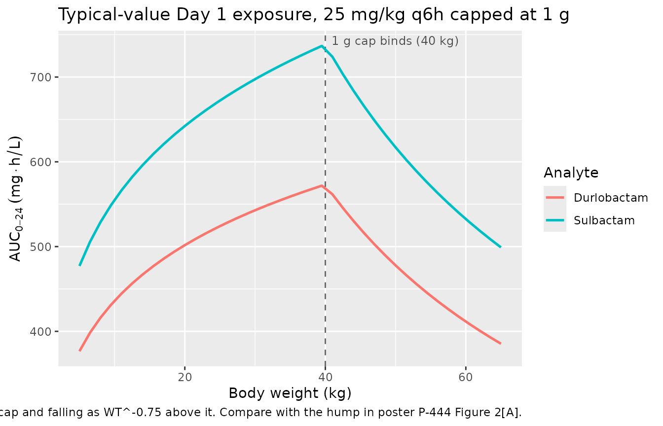
The 1 g cap produces a predictable inflection in exposure

At steady state, exposure over one dosing interval is exactly dose / clearance. For an uncapped mg/kg dose that is $\mathrm{WT}\,/\,\mathrm{WT}^{0.75} = \mathrm{WT}^{0.25}$ — slowly rising with size. Once the 1 g cap binds (at 1000 / 25 = 40 kg) the dose is constant and exposure falls as $\mathrm{WT}^{-0.75}$. The model therefore predicts a peak in exposure at exactly 40 kg, which is visible as the hump in the poster’s own Figure 2[A].

wt_grid <- tibble::as_tibble(c(
  list(id = seq_len(41L), WT = seq(5, 65, length.out = 41L)),
  POSTER_COVS
)) |>
  dplyr::mutate(dose_mg = pmin(25 * WT, 1000))

# q6h out to 48 h so BOTH Day 1 (what the poster plots) and a steady-state
# dosing interval (where the allometry is exact) come from one solve.
cap_events <- dplyr::bind_rows(
  wt_grid |>
    tidyr::crossing(time = seq(0, 42, by = 6), cmt = c("central", "central_sbt")) |>
    dplyr::mutate(evid = 1L, amt = dose_mg, rate = dose_mg / 3,
                  dvid = NA_integer_),
  wt_grid |>
    tidyr::crossing(time = seq(0, 48, by = 0.05)) |>
    dplyr::mutate(evid = 0L, amt = NA_real_, rate = NA_real_,
                  cmt = "central", dvid = 1L)
) |>
  dplyr::arrange(id, time, dplyr::desc(evid))

cap_sim <- solve_typical(mod_allo, cap_events, keep = c("WT", "dose_mg"))

cap_auc <- cap_sim |>
  dplyr::filter(!is.na(Cc)) |>
  dplyr::group_by(id, WT, dose_mg) |>
  dplyr::summarise(
    Durlobactam = trapz(time[time <= 24], Cc[time <= 24]),
    Sulbactam   = trapz(time[time <= 24], Cc_sbt[time <= 24]),
    ss_dur      = trapz(time[time >= 42], Cc[time >= 42]),
    .groups     = "drop"
  )

peak_wt <- cap_auc$WT[which.max(cap_auc$Durlobactam)]

cap_auc |>
  tidyr::pivot_longer(c(Durlobactam, Sulbactam),
                      names_to = "Analyte", values_to = "auc") |>
  ggplot(aes(WT, auc, colour = Analyte)) +
  geom_vline(xintercept = 40, linetype = "dashed", colour = "grey40") +
  geom_line(linewidth = 0.9) +
  annotate("text", x = 40, y = Inf, label = "1 g cap binds (40 kg)",
           hjust = -0.05, vjust = 1.6, size = 3.2, colour = "grey30") +
  labs(
    x = "Body weight (kg)", y = expression(AUC[0-24]~(mg%.%h/L)),
    title = "Typical-value Day 1 exposure, 25 mg/kg q6h capped at 1 g",
    caption = paste(
      "Rising as WT^0.25 below the cap and falling as WT^-0.75 above it.",
      "Compare with the hump in poster P-444 Figure 2[A]."
    )
  )

below <- cap_auc |> dplyr::filter(WT <= 40)
above <- cap_auc |> dplyr::filter(WT >= 40)

slope <- function(df, col) {
  stats::coef(stats::lm(log(df[[col]]) ~ log(df$WT)))[[2]]
}

slopes <- tibble::tibble(
  "Weight range"          = rep(c("<= 40 kg (mg/kg dosing)",
                                  ">= 40 kg (1 g cap)"), 2),
  "Exposure measure"      = rep(c("Steady-state AUC over one interval",
                                  "Day 1 AUC0-24"), each = 2),
  "Fitted log-log slope"  = c(slope(below, "ss_dur"), slope(above, "ss_dur"),
                              slope(below, "Durlobactam"),
                              slope(above, "Durlobactam")),
  "Allometric prediction" = c(0.25, -0.75, NA, NA)
)

knitr::kable(
  slopes, digits = 4,
  caption = paste(
    "Durlobactam exposure versus body weight. At steady state AUC over one",
    "dosing interval is exactly dose / clearance, so the slopes are exactly",
    "the allometric predictions. Day 1 AUC0-24 is shallower below the cap and",
    "steeper above it because accumulation is not yet complete at 24 h and the",
    "elimination rate constant itself falls with weight (kel = CL / Vc scales",
    "as WT^-0.25), so a larger child retains proportionally more drug at 24 h."
  )
)

Durlobactam exposure versus body weight. At steady state AUC over one dosing interval is exactly dose / clearance, so the slopes are exactly the allometric predictions. Day 1 AUC0-24 is shallower below the cap and steeper above it because accumulation is not yet complete at 24 h and the elimination rate constant itself falls with weight (kel = CL / Vc scales as WT^-0.25), so a larger child retains proportionally more drug at 24 h.

Weight range	Exposure measure	Fitted log-log slope	Allometric prediction
<= 40 kg (mg/kg dosing)	Steady-state AUC over one interval	0.2499	0.25
>= 40 kg (1 g cap)	Steady-state AUC over one interval	-0.7508	-0.75
<= 40 kg (mg/kg dosing)	Day 1 AUC0-24	0.2009	NA
>= 40 kg (1 g cap)	Day 1 AUC0-24	-0.8179	NA

# EXACT gate on the quantity that is exact: at steady state AUCtau = dose / CL,
# so the two limbs must have the allometric exponents to within trapezoidal
# integration error.
stopifnot(
  abs(slope(below, "ss_dur") -  0.25) < 0.005,
  abs(slope(above, "ss_dur") - -0.75) < 0.005
)

# The peak sits on the cap weight. Grid spacing is 1.5 kg, so the nearest grid
# point to 40 is the tightest this can be.
stopifnot(abs(peak_wt - 40) <= 1.5)

# Day 1 is a derived, non-exact quantity; gate its SHAPE (rising then falling,
# with the deviations from 0.25 / -0.75 in the direction incomplete
# accumulation predicts) rather than pinning it to one run's value.
stopifnot(
  slope(below, "Durlobactam") > 0.15,
  slope(below, "Durlobactam") < 0.25,
  slope(above, "Durlobactam") < -0.75,
  slope(above, "Durlobactam") > -0.95
)

Comparing the two approaches (cf. Figures 2 and 3)

The poster’s headline modelling result is that the Allometry + CL_CR model predicts lower exposures than Adult with Allometry, which is why the latter was chosen as the more conservative basis for dose selection.

two_sim <- dplyr::bind_rows(
  solve_typical(mod_allo, cap_events, keep = c("WT", "dose_mg")) |>
    dplyr::mutate(model = "Adult with Allometry"),
  solve_typical(mod_crcl, cap_events, keep = c("WT", "dose_mg")) |>
    dplyr::mutate(model = "Allometry + CLcr")
)

two_auc <- two_sim |>
  dplyr::filter(!is.na(Cc)) |>
  dplyr::group_by(model, id, WT) |>
  dplyr::summarise(
    Durlobactam = trapz(time[time <= 24], Cc[time <= 24]),      # Day 1, as plotted
    Sulbactam   = trapz(time[time <= 24], Cc_sbt[time <= 24]),
    ss_dur      = trapz(time[time >= 42], Cc[time >= 42]),      # steady-state interval
    ss_sbt      = trapz(time[time >= 42], Cc_sbt[time >= 42]),
    vc          = dplyr::first(vc),
    .groups     = "drop"
  )

two_auc |>
  tidyr::pivot_longer(c(Durlobactam, Sulbactam),
                      names_to = "Analyte", values_to = "auc") |>
  ggplot(aes(WT, auc, colour = model)) +
  geom_line(linewidth = 0.9) +
  facet_wrap(~Analyte, scales = "free_y") +
  labs(
    x = "Body weight (kg)", y = expression(AUC[0-24]~(mg%.%h/L)),
    colour = NULL,
    title = "Typical-value Day 1 exposure under the poster's two approaches",
    caption = "Compare with poster P-444 Figure 2 (upper) versus Figure 3 (lower)."
  ) +
  theme(legend.position = "bottom")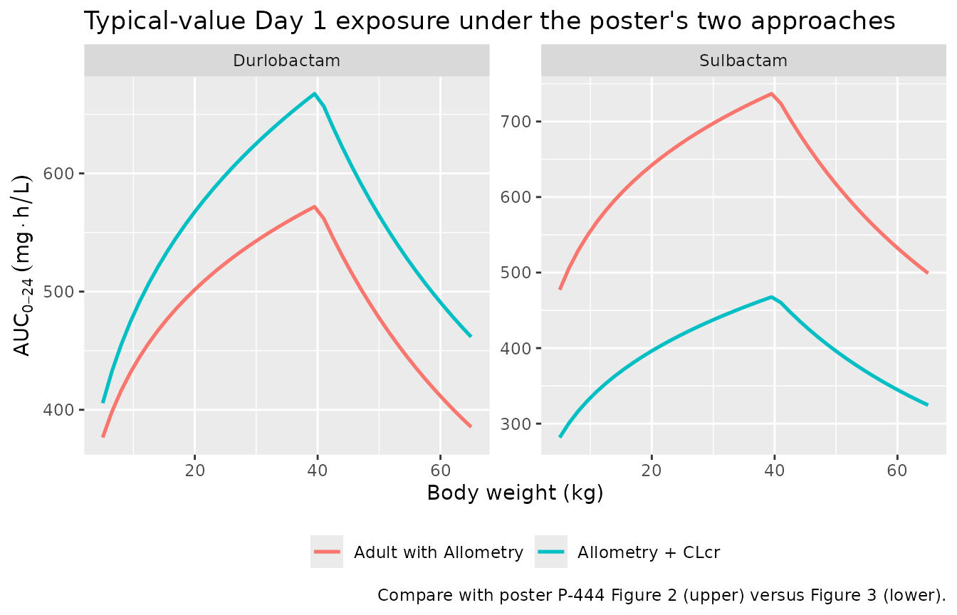

wide <- two_auc |>
  dplyr::select(model, id, WT, Durlobactam, Sulbactam, ss_dur, ss_sbt) |>
  tidyr::pivot_longer(c(Durlobactam, Sulbactam, ss_dur, ss_sbt),
                      names_to = "measure", values_to = "auc") |>
  tidyr::pivot_wider(names_from = model, values_from = auc) |>
  dplyr::mutate(ratio = `Allometry + CLcr` / `Adult with Allometry`)

ratio_tab <- wide |>
  dplyr::group_by(measure) |>
  dplyr::summarise(ratio = stats::median(ratio), .groups = "drop") |>
  dplyr::mutate(
    Analyte  = ifelse(grepl("dur|Durlo", measure), "Durlobactam", "Sulbactam"),
    Exposure = ifelse(grepl("^ss_", measure),
                      "Steady-state AUC over one interval", "Day 1 AUC0-24"),
    Exact    = ifelse(grepl("^ss_", measure),
                      ifelse(grepl("dur", measure), 1, 1 - 0.444), NA_real_)
  )

ratio_tab |>
  dplyr::select(Analyte, Exposure,
                "Median ratio (CLcr model / allometry model)" = ratio,
                "Exact algebraic value" = Exact) |>
  dplyr::arrange(Analyte, Exposure) |>
  knitr::kable(
    digits  = 4,
    caption = paste(
      "Poster P-444 Results: 'Compared to the adult with allometry model, the",
      "adult with allometry + CLCR model predicted lower SUD exposures.' At a",
      "common CLcr, the steady-state ratio is exact algebra; the Day 1 ratio",
      "is not, because the two models also differ in central volume."
    )
  )

Poster P-444 Results: ‘Compared to the adult with allometry model, the adult with allometry + CLCR model predicted lower SUD exposures.’ At a common CLcr, the steady-state ratio is exact algebra; the Day 1 ratio is not, because the two models also differ in central volume.

Analyte	Exposure	Median ratio (CLcr model / allometry model)	Exact algebraic value
Durlobactam	Day 1 AUC0-24	1.1602	NA
Durlobactam	Steady-state AUC over one interval	1.0002	1.000
Sulbactam	Day 1 AUC0-24	0.6313	NA
Sulbactam	Steady-state AUC over one interval	0.5560	0.556

At steady state, exposure over one dosing interval is dose / clearance and does not depend on volume at all, which makes the two steady-state ratios exact:

• Durlobactam’s bacteremia effect acts on central volume (+3.32), not clearance, and durlobactam carries no region or infection effect on clearance. Removing those covariates leaves steady-state durlobactam exposure exactly unchanged — ratio 1.
• Sulbactam’s bacteremia effect acts on clearance (-0.444). Removing it raises clearance by 1 / (1 - 0.444), so exposure falls by exactly 0.556.

ss <- ratio_tab |> dplyr::filter(grepl("^ss_", measure))
stopifnot(nrow(ss) == 2L, max(abs(ss$ratio - ss$Exact)) < 1e-3)

# The volume ratio is likewise exact: 1 + 3.32 = 4.32.
vc_ratio <- two_auc |>
  dplyr::select(model, id, vc) |>
  tidyr::pivot_wider(names_from = model, values_from = vc) |>
  dplyr::summarise(r = stats::median(`Adult with Allometry` / `Allometry + CLcr`)) |>
  dplyr::pull(r)
stopifnot(abs(vc_ratio - 4.32) < 1e-6)

# The poster's claim -- lower exposures under Allometry + CLcr -- is reproduced
# for sulbactam on BOTH measures.
stopifnot(all(ratio_tab$ratio[ratio_tab$Analyte == "Sulbactam"] < 0.7))

Durlobactam does not reproduce the poster’s direction, and that is informative rather than a defect. On Day 1 the ratio comes out above 1: the “Adult with Allometry” model gives durlobactam a 4.32-fold larger central volume, so its elimination rate constant kel = CL / Vc is 4.32-fold smaller and proportionally more drug is still in the body at 24 h, depressing its AUC_0-24. At steady state that transient washes out and the ratio returns to exactly 1. Either way, at a common CL_CR the two models cannot make durlobactam exposure lower under “Allometry + CL_CR”, because durlobactam clearance is identical between them. Since the poster’s Figure 3[A] does show lower durlobactam exposure, the two models must have been driven with different renal function — which is what their names imply and what the Rhodin formula in the abstract was for. That formula is not in either source on disk, so this vignette does not guess at it. See Assumptions and deviations.

Virtual cohort and stochastic simulation

set.seed(20260910)

N_PER_ARM <- 150L   # under the 200-per-arm validation-vignette cap

# Weight bands spanning the pediatric range. These are illustrative body-weight
# strata, NOT an age-to-weight mapping taken from the sources -- see
# *Assumptions and deviations*.
bands <- tibble::tribble(
  ~band,        ~wt_lo, ~wt_hi, ~mg_per_kg, ~tau,
  "2-5 kg",       2,      5,     20,         12,
  "5-10 kg",      5,     10,     25,          6,
  "10-20 kg",    10,     20,     25,          6,
  "20-40 kg",    20,     40,     25,          6,
  "40-65 kg",    40,     65,     25,          6
)

cohort <- bands |>
  dplyr::mutate(row = dplyr::row_number()) |>
  tidyr::crossing(k = seq_len(N_PER_ARM)) |>
  dplyr::mutate(
    id      = (row - 1L) * 1000L + k,
    WT      = stats::runif(dplyr::n(), wt_lo, wt_hi),
    dose_mg = pmin(mg_per_kg * WT, 1000)
  ) |>
  dplyr::select(id, band, tau, WT, dose_mg)

for (nm in names(POSTER_COVS)) cohort[[nm]] <- POSTER_COVS[[nm]]

cohort_events <- dplyr::bind_rows(
  # Dosing times differ by band (q6h or q12h), so cross with every hour and
  # keep the multiples of that subject's interval.
  cohort |>
    tidyr::crossing(time = 0:23) |>
    dplyr::filter(time %% tau == 0) |>
    tidyr::crossing(cmt = c("central", "central_sbt")) |>
    dplyr::mutate(evid = 1L, amt = dose_mg, rate = dose_mg / 3,
                  dvid = NA_integer_),
  cohort |>
    tidyr::crossing(time = seq(0, 24, by = 0.25)) |>
    dplyr::mutate(evid = 0L, amt = NA_real_, rate = NA_real_,
                  cmt = "central", dvid = 1L)
) |>
  dplyr::arrange(id, time, dplyr::desc(evid))

stopifnot(nrow(cohort) == 5L * N_PER_ARM)

sim <- rxode2::rxSolve(
  mod_allo, events = cohort_events,
  keep = c("band", "WT", "dose_mg"),
  useLinCmt = FALSE
) |>
  as.data.frame()

dplyr::glimpse(sim[, c("id", "time", "Cc", "Cc_sbt", "Celf", "Celf_sbt",
                       "cl", "cl_sbt", "band", "WT")])
#> Rows: 72,750
#> Columns: 10
#> $ id       <int> 1, 1, 1, 1, 1, 1, 1, 1, 1, 1, 1, 1, 1, 1, 1, 1, 1, 1, 1, 1, 1…
#> $ time     <dbl> 0.00, 0.25, 0.50, 0.75, 1.00, 1.25, 1.50, 1.75, 2.00, 2.25, 2…
#> $ Cc       <dbl> 0.000000, 1.499996, 2.818940, 3.988123, 5.031479, 5.967595, 6…
#> $ Cc_sbt   <dbl> 0.000000, 4.100260, 7.283152, 9.911786, 12.167038, 14.144321,…
#> $ Celf     <dbl> 0.0000000, 0.5579985, 1.0486458, 1.4835818, 1.8717100, 2.2199…
#> $ Celf_sbt <dbl> 0.000000, 2.185439, 3.881920, 5.282982, 6.485031, 7.538923, 8…
#> $ cl       <dbl> 0.866039, 0.866039, 0.866039, 0.866039, 0.866039, 0.866039, 0…
#> $ cl_sbt   <dbl> 0.4312815, 0.4312815, 0.4312815, 0.4312815, 0.4312815, 0.4312…
#> $ band     <chr> "2-5 kg", "2-5 kg", "2-5 kg", "2-5 kg", "2-5 kg", "2-5 kg", "…
#> $ WT       <dbl> 2.021976, 2.021976, 2.021976, 2.021976, 2.021976, 2.021976, 2…

Simulated pediatric exposures against the adult reference range

Poster P-444 Table 1 gives the adult median and 5th-95th percentile exposures that the pediatric regimens were targeted to sit inside. The poster’s stated result is that

The adult with allometry model provided SUD exposures that were predominantly contained within the 5th and 95th percentiles of adult exposures based on AUC_0-24

adult_exposure <- tibble::tribble(
  ~Analyte,      ~Parameter,   ~day, ~median, ~p05,  ~p95,
  "Sulbactam",   "AUC0-24",     1,    441,     196,   1170,
  "Sulbactam",   "AUC0-24",     3,    469,     192,   1710,
  "Sulbactam",   "Cmax",        1,     30.0,    14.7,   75.9,
  "Sulbactam",   "Cmax",        3,     29.5,    14.3,   88.8,
  "Durlobactam", "AUC0-24",     1,    442,     277,    904,
  "Durlobactam", "AUC0-24",     3,    479,     239,   1180,
  "Durlobactam", "Cmax",        1,     30.3,    18.4,   58.9,
  "Durlobactam", "Cmax",        3,     30.5,    17.3,   65.0
)

adult_exposure |>
  dplyr::transmute(
    Analyte, Parameter, Day = day,
    "Median (5th-95th percentile)" =
      paste0(median, " (", p05, "-", p95, ")")
  ) |>
  knitr::kable(
    caption = paste(
      "Poster P-444 Table 1: adult sulbactam and durlobactam exposures on Day 1",
      "and Day 3. AUC0-24 in h*mg/L, Cmax in mg/L."
    )
  )

Poster P-444 Table 1: adult sulbactam and durlobactam exposures on Day 1 and Day 3. AUC0-24 in h*mg/L, Cmax in mg/L.

Analyte	Parameter	Day	Median (5th-95th percentile)
Sulbactam	AUC0-24	1	441 (196-1170)
Sulbactam	AUC0-24	3	469 (192-1710)
Sulbactam	Cmax	1	30 (14.7-75.9)
Sulbactam	Cmax	3	29.5 (14.3-88.8)
Durlobactam	AUC0-24	1	442 (277-904)
Durlobactam	AUC0-24	3	479 (239-1180)
Durlobactam	Cmax	1	30.3 (18.4-58.9)
Durlobactam	Cmax	3	30.5 (17.3-65)

env <- adult_exposure |>
  dplyr::filter(Parameter == "AUC0-24", day == 1) |>
  dplyr::select(Analyte, p05, p95)

ped_auc <- sim |>
  dplyr::filter(!is.na(Cc)) |>
  dplyr::group_by(band, id) |>
  dplyr::summarise(Durlobactam = trapz(time, Cc),
                   Sulbactam   = trapz(time, Cc_sbt), .groups = "drop") |>
  tidyr::pivot_longer(c(Durlobactam, Sulbactam),
                      names_to = "Analyte", values_to = "auc") |>
  dplyr::left_join(env, by = "Analyte")

band_summary <- ped_auc |>
  dplyr::group_by(Analyte, band, p05, p95) |>
  dplyr::summarise(
    med = stats::median(auc),
    pct_inside = 100 * mean(auc >= p05 & auc <= p95),
    .groups = "drop"
  ) |>
  dplyr::mutate(
    median_inside = med >= p05 & med <= p95,
    # The 2-5 kg band is the neonatal stratum, where BSA-normalized renal
    # function is far below the adult reference. Reproducing it needs the
    # Rhodin maturation function, which is not in either source on disk, so
    # it is recorded as a deviation rather than gated. See Errata.
    deviation = band == "2-5 kg"
  )

band_summary |>
  dplyr::transmute(
    Analyte,
    "Weight band"             = band,
    "Median AUC0-24"          = med,
    "% inside adult 5th-95th" = pct_inside,
    "Median inside adult range" = ifelse(median_inside, "yes", "no"),
    "Deviation"               = ifelse(deviation, "yes", "")
  ) |>
  knitr::kable(
    digits  = 1,
    caption = paste(
      "Simulated Day 1 AUC0-24 (h*mg/L) by weight band under the 'Adult with",
      "Allometry' model, against the adult 5th-95th percentile range of poster",
      "P-444 Table 1. The neonatal 2-5 kg band is flagged as a deviation: it",
      "needs the renal-maturation function this vignette cannot reproduce."
    )
  )

Simulated Day 1 AUC0-24 (h*mg/L) by weight band under the ‘Adult with Allometry’ model, against the adult 5th-95th percentile range of poster P-444 Table 1. The neonatal 2-5 kg band is flagged as a deviation: it needs the renal-maturation function this vignette cannot reproduce.

Analyte	Weight band	Median AUC0-24	% inside adult 5th-95th	Median inside adult range	Deviation
Durlobactam	10-20 kg	488.4	98.0	yes
Durlobactam	2-5 kg	143.0	0.7	no	yes
Durlobactam	20-40 kg	538.2	96.7	yes
Durlobactam	40-65 kg	447.6	92.0	yes
Durlobactam	5-10 kg	408.5	88.7	yes
Sulbactam	10-20 kg	578.8	94.0	yes
Sulbactam	2-5 kg	172.3	40.0	no	yes
Sulbactam	20-40 kg	657.7	93.3	yes
Sulbactam	40-65 kg	578.7	98.7	yes
Sulbactam	5-10 kg	533.2	96.0	yes

gated <- band_summary |> dplyr::filter(!deviation)

# Guard against a vacuous gate: confirm there are rows to test (all(logical(0))
# is TRUE, so a label mismatch would silently pass).
stopifnot(nrow(gated) == 8L)

# The poster's claim is about the CENTRE of the pediatric distribution sitting
# inside the adult range, so assert on band medians -- a cohort's extremes are
# not reproducible across rxode2 versions or solver thread counts.
stopifnot(all(gated$median_inside))

# "Predominantly contained" is qualitative; require a clear majority per band
# rather than a threshold read off one run.
stopifnot(all(gated$pct_inside > 55))

The four bands from 5 kg upward reproduce the poster’s headline result: the median simulated pediatric exposure sits inside the adult 5th-95th percentile range for both analytes, and the large majority of individual subjects do too.

The neonatal 2-5 kg band falls below the adult range for both analytes, and this is expected rather than a transcription error. That band is dosed 20 mg/kg q12h (two doses a day rather than four), and the model as packaged scales clearance by weight alone — so at a fixed CL_CR of 100 mL/min/1.73 m^2 it gives a term neonate a fully mature renal clearance per kilogram. The poster instead assigned each simulated subject a Rhodin-derived renal function, which in a neonate is a fraction of the adult value. The sensitivity below shows how far renal function has to fall to close the gap.

neo <- tibble::as_tibble(c(
  list(id = seq_len(6L), WT = 3.5),
  utils::modifyList(POSTER_COVS, list(CRCL = NULL, RENALIMP_SEV = NULL))
)) |>
  dplyr::mutate(
    CRCL         = c(100, 75, 50, 30, 20, 10),
    RENALIMP_SEV = as.numeric(CRCL < 30)
  )

neo_ev  <- make_events(neo, dose_mg = 20 * 3.5, tau = 12, tmax = 24, by = 0.05)
neo_sim <- solve_typical(mod_allo, neo_ev, keep = c("WT", "CRCL"))

neo_tab <- neo_sim |>
  dplyr::filter(!is.na(Cc)) |>
  dplyr::group_by(CRCL) |>
  dplyr::summarise(Durlobactam = trapz(time, Cc),
                   Sulbactam   = trapz(time, Cc_sbt), .groups = "drop") |>
  # dplyr returns groups in ascending CRCL order; make that explicit so the
  # monotonicity assertion below cannot silently invert.
  dplyr::arrange(CRCL) |>
  dplyr::mutate(
    `Durlobactam inside adult range` =
      ifelse(Durlobactam >= 277 & Durlobactam <= 904, "yes", "no"),
    `Sulbactam inside adult range` =
      ifelse(Sulbactam >= 196 & Sulbactam <= 1170, "yes", "no")
  )

neo_tab |>
  dplyr::rename("CLcr (mL/min/1.73 m^2)" = CRCL) |>
  knitr::kable(
    digits  = 1,
    caption = paste(
      "Typical-value Day 1 AUC0-24 (h*mg/L) for a 3.5 kg term neonate on",
      "20 mg/kg q12h, as a function of the renal function assigned. The adult",
      "reference ranges are 277-904 (durlobactam) and 196-1170 (sulbactam).",
      "Exposure enters the adult range once renal function drops well below",
      "the adult reference, which is what a maturation function supplies."
    )
  )

Typical-value Day 1 AUC0-24 (h*mg/L) for a 3.5 kg term neonate on 20 mg/kg q12h, as a function of the renal function assigned. The adult reference ranges are 277-904 (durlobactam) and 196-1170 (sulbactam). Exposure enters the adult range once renal function drops well below the adult reference, which is what a maturation function supplies.

CLcr (mL/min/1.73 m^2)	Durlobactam	Sulbactam	Durlobactam inside adult range	Sulbactam inside adult range
10	432.2	639.9	yes	yes
20	411.7	615.2	yes	yes
30	206.6	277.8	no	yes
50	184.4	244.9	no	yes
75	163.3	211.1	no	yes
100	147.0	184.0	no	no

# Deterministic typical-value monotonicity. The table is sorted by ASCENDING
# CLcr, so exposure must be strictly DECREASING down the rows.
stopifnot(
  nrow(neo_tab) == 6L,
  all(diff(neo_tab$Durlobactam) < 0),
  all(diff(neo_tab$Sulbactam)   < 0),
  # At the adult reference CLcr the neonate falls below the adult range ...
  neo_tab$`Durlobactam inside adult range`[neo_tab$CRCL == 100] == "no",
  # ... and the gap IS closable by renal function alone, which is the point.
  any(neo_tab$`Durlobactam inside adult range` == "yes")
)

ped_auc |>
  ggplot(aes(band, auc)) +
  geom_hline(aes(yintercept = p05), linetype = "dashed", colour = "grey40") +
  geom_hline(aes(yintercept = p95), linetype = "dashed", colour = "grey40") +
  geom_boxplot(outlier.size = 0.5, fill = "steelblue", alpha = 0.35) +
  facet_wrap(~Analyte, scales = "free_y") +
  labs(
    x = "Body-weight band", y = expression(AUC[0-24]~(mg%.%h/L)),
    title = "Simulated pediatric Day 1 exposure versus the adult reference range",
    caption = paste(
      "Dashed lines are the adult 5th and 95th percentiles of poster P-444",
      "Table 1. Compare with poster P-444 Figure 2[A] and [B]."
    )
  ) +
  theme(axis.text.x = element_text(angle = 30, hjust = 1))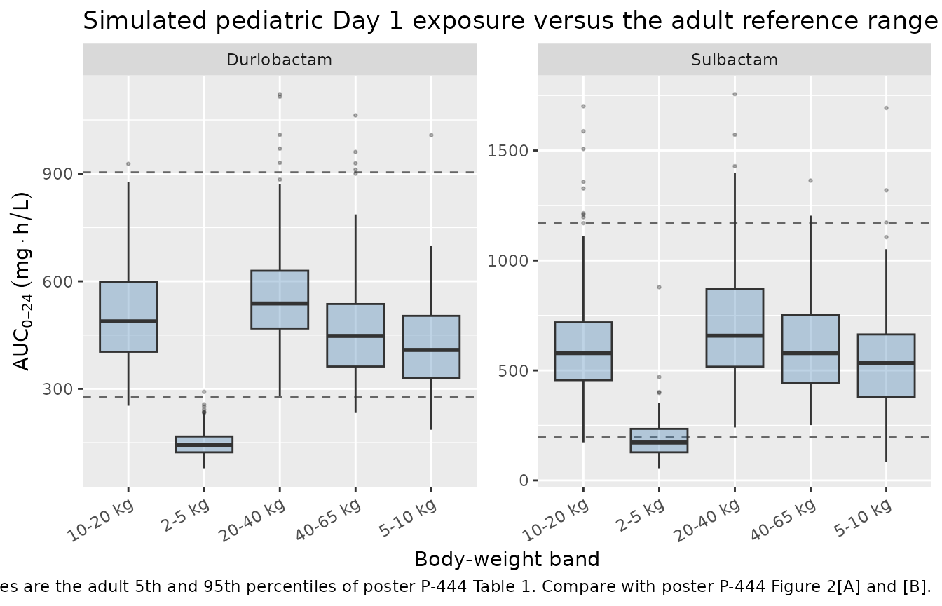

PKNCA validation

#' Run PKNCA over 0-24 h for one concentration column of a simulation frame.
nca_for <- function(sim_df, conc_col, dose_df) {
  sim_nca <- sim_df |>
    dplyr::rename(Cc_use = dplyr::all_of(conc_col)) |>
    dplyr::filter(!is.na(Cc_use)) |>
    dplyr::select(id, time, Cc = Cc_use, band)

  # Guarantee a time-zero row per (band, id); pre-dose IV concentration is 0.
  sim_nca <- dplyr::bind_rows(
    sim_nca,
    sim_nca |> dplyr::distinct(id, band) |> dplyr::mutate(time = 0, Cc = 0)
  ) |>
    dplyr::distinct(band, id, time, .keep_all = TRUE) |>
    dplyr::arrange(id, time)

  conc_obj <- PKNCA::PKNCAconc(sim_nca, Cc ~ time | band + id,
                               concu = "mg/L", timeu = "h")
  dose_obj <- PKNCA::PKNCAdose(dose_df, amt ~ time | band + id, doseu = "mg")

  intervals <- data.frame(start = 0, end = 24,
                          cmax = TRUE, tmax = TRUE, auclast = TRUE)

  PKNCA::pk.nca(PKNCA::PKNCAdata(conc_obj, dose_obj, intervals = intervals))
}

dose_df <- cohort_events |>
  dplyr::filter(evid == 1, cmt == "central") |>
  dplyr::select(id, time, amt, band)

nca_dur <- nca_for(sim, "Cc", dose_df)
nca_sbt <- nca_for(sim, "Cc_sbt", dose_df)

stopifnot(nrow(as.data.frame(nca_dur)) > 0,
          nrow(as.data.frame(nca_sbt)) > 0)

# Cross-check PKNCA against the independent trapezoidal AUC used above. Two
# implementations of the same integral over the same grid must agree closely.
pknca_auc <- as.data.frame(nca_dur) |>
  dplyr::filter(PPTESTCD == "auclast") |>
  dplyr::select(band, id, pknca = PPORRES)

chk <- ped_auc |>
  dplyr::filter(Analyte == "Durlobactam") |>
  dplyr::select(band, id, trapz = auc) |>
  dplyr::inner_join(pknca_auc, by = c("band", "id")) |>
  dplyr::mutate(pct_diff = 100 * (pknca - trapz) / trapz)

stopifnot(
  nrow(chk) == 5L * N_PER_ARM,
  max(abs(chk$pct_diff)) < 0.5
)

tibble::tibble(
  "Subjects compared"          = nrow(chk),
  "Max |% difference|"         = max(abs(chk$pct_diff)),
  "Median |% difference|"      = stats::median(abs(chk$pct_diff))
) |>
  knitr::kable(
    digits  = 4,
    caption = paste(
      "PKNCA auclast over 0-24 h against the independent trapezoidal integral,",
      "per simulated subject."
    )
  )

PKNCA auclast over 0-24 h against the independent trapezoidal integral, per simulated subject.

Subjects compared	Max |% difference|	Median |% difference|
750	0.0939	0.0165

Adult exposures on Day 1 versus Day 3 (cf. Table 1)

At 75 kg the pediatric model reduces to the adult model, so the packaged model can reproduce the poster’s own adult reference column. The poster’s stated conclusion from Table 1 is a lack of accumulation — and a Day 3 / Day 1 ratio is insensitive to the (unreported) covariate mix of the adult post-hoc population, which the absolute values are not.

Table 1 describes the real adult Phase 2/3 population, whose infection-type mix the poster does not report — so it is not the bacteremia setting used for the pediatric simulations. Both settings are shown below, because the contrast between them is itself a structural check.

adult_setting <- function(bacteremia) {
  covs <- utils::modifyList(POSTER_COVS, list(DIS_BACTEREMIA = bacteremia))
  subj <- tibble::as_tibble(c(list(id = 1L, WT = 75), covs))
  s <- solve_typical(mod_allo, make_events(subj, 1000, 6, 72, by = 0.05),
                     keep = "WT") |>
    dplyr::filter(!is.na(Cc))
  d1 <- s$time <= 24
  d3 <- s$time >= 48
  tibble::tibble(
    setting  = if (bacteremia == 1) "Bacteremia (pediatric-simulation setting)"
               else "Uninfected reference",
    vc_dur   = s$vc[1],
    dur_d1   = trapz(s$time[d1], s$Cc[d1]),
    dur_d3   = trapz(s$time[d3], s$Cc[d3]),
    sbt_d1   = trapz(s$time[d1], s$Cc_sbt[d1]),
    sbt_d3   = trapz(s$time[d3], s$Cc_sbt[d3]),
    dur_cmax_d1 = max(s$Cc[d1]),      dur_cmax_d3 = max(s$Cc[d3]),
    sbt_cmax_d1 = max(s$Cc_sbt[d1]),  sbt_cmax_d3 = max(s$Cc_sbt[d3])
  )
}

acc <- dplyr::bind_rows(adult_setting(0), adult_setting(1))

acc_tab <- acc |>
  dplyr::transmute(
    Setting = setting,
    "Durlobactam Vc (L)"    = vc_dur,
    "Durlobactam AUC D3/D1" = dur_d3 / dur_d1,
    "Durlobactam Cmax D3/D1"= dur_cmax_d3 / dur_cmax_d1,
    "Sulbactam AUC D3/D1"   = sbt_d3 / sbt_d1,
    "Sulbactam Cmax D3/D1"  = sbt_cmax_d3 / sbt_cmax_d1
  )

dplyr::bind_rows(
  acc_tab,
  tibble::tibble(
    Setting = "Poster P-444 Table 1 (observed adults)",
    `Durlobactam Vc (L)`     = NA_real_,
    `Durlobactam AUC D3/D1`  = 479 / 442,
    `Durlobactam Cmax D3/D1` = 30.5 / 30.3,
    `Sulbactam AUC D3/D1`    = 469 / 441,
    `Sulbactam Cmax D3/D1`   = 29.5 / 30.0
  )
) |>
  knitr::kable(
    digits  = 3,
    caption = paste(
      "Day 3 / Day 1 accumulation ratios at the adult 1 g / 1 g q6h regimen.",
      "Poster P-444 Results: the Table 1 exposures 'demonstrate lack of",
      "accumulation'. The uninfected reference reproduces that; the bacteremia",
      "setting accumulates more because its 4.32-fold larger central volume",
      "lengthens the effective half-life."
    )
  )

Day 3 / Day 1 accumulation ratios at the adult 1 g / 1 g q6h regimen. Poster P-444 Results: the Table 1 exposures ‘demonstrate lack of accumulation’. The uninfected reference reproduces that; the bacteremia setting accumulates more because its 4.32-fold larger central volume lengthens the effective half-life.

Setting	Durlobactam Vc (L)	Durlobactam AUC D3/D1	Durlobactam Cmax D3/D1	Sulbactam AUC D3/D1	Sulbactam Cmax D3/D1
Uninfected reference	12.5	1.036	1.000	1.018	1.000
Bacteremia (pediatric-simulation setting)	54.0	1.251	1.025	1.199	1.014
Poster P-444 Table 1 (observed adults)	NA	1.084	1.007	1.063	0.983

ref  <- acc |> dplyr::filter(setting == "Uninfected reference")
bact <- acc |> dplyr::filter(setting != "Uninfected reference")
stopifnot(nrow(ref) == 1L, nrow(bact) == 1L)

# 1. At the uninfected reference the model shows the near-absence of
#    accumulation that Table 1 reports (published ratios 1.06-1.08 for AUC and
#    0.98-1.01 for Cmax).
stopifnot(
  abs(ref$dur_d3 / ref$dur_d1 - 1) < 0.10,
  abs(ref$sbt_d3 / ref$sbt_d1 - 1) < 0.10,
  abs(ref$dur_cmax_d3 / ref$dur_cmax_d1 - 1) < 0.02,
  abs(ref$sbt_cmax_d3 / ref$sbt_cmax_d1 - 1) < 0.02
)

# 2. Structural consequence of the bacteremia Vc shift: a larger volume at the
#    same clearance lengthens the effective half-life, so accumulation MUST be
#    greater. Deterministic typical values, so a plain inequality is safe.
stopifnot(
  bact$vc_dur / ref$vc_dur > 4,
  bact$dur_d3 / bact$dur_d1 > ref$dur_d3 / ref$dur_d1,
  bact$sbt_d3 / bact$sbt_d1 > ref$sbt_d3 / ref$sbt_d1
)

# 3. Steady state is a covariate-independent anchor: Day 3 exposure is
#    dose / CL regardless of volume, so the two settings must agree on
#    durlobactam Day 3 (durlobactam has no infection effect on clearance).
stopifnot(abs(bact$dur_d3 / ref$dur_d3 - 1) < 0.01)

tibble::tibble(
  Analyte   = c("Durlobactam", "Durlobactam", "Sulbactam", "Sulbactam"),
  Parameter = c("AUC0-24 (Day 3)", "Cmax (Day 3)",
                "AUC0-24 (Day 3)", "Cmax (Day 3)"),
  Simulated = c(ref$dur_d3, ref$dur_cmax_d3, ref$sbt_d3, ref$sbt_cmax_d3),
  Published = c(479, 30.5, 469, 29.5)
) |>
  dplyr::mutate(`% difference` = 100 * (Simulated - Published) / Published) |>
  dplyr::rename("Poster Table 1 median" = Published) |>
  knitr::kable(
    digits  = 1,
    caption = paste(
      "Typical-value adult Day 3 exposures at 1 g / 1 g q6h (75 kg,",
      "non-East-Asian, CLcr 100, uninfected reference) against the poster's",
      "Table 1 medians. This is a DEVIATION table, not a gate. Durlobactam is",
      "close; sulbactam is under-predicted because every infection-type",
      "covariate in the adult model REDUCES sulbactam clearance by 16-44%, and",
      "the Table 1 population is entirely infected patients whose mix the",
      "poster does not report."
    )
  )

Typical-value adult Day 3 exposures at 1 g / 1 g q6h (75 kg, non-East-Asian, CLcr 100, uninfected reference) against the poster’s Table 1 medians. This is a DEVIATION table, not a gate. Durlobactam is close; sulbactam is under-predicted because every infection-type covariate in the adult model REDUCES sulbactam clearance by 16-44%, and the Table 1 population is entirely infected patients whose mix the poster does not report.

Analyte	Parameter	Simulated	Poster Table 1 median	% difference
Durlobactam	AUC0-24 (Day 3)	428.7	479.0	-10.5
Durlobactam	Cmax (Day 3)	29.9	30.5	-2.1
Sulbactam	AUC0-24 (Day 3)	296.3	469.0	-36.8
Sulbactam	Cmax (Day 3)	21.9	29.5	-25.9

Assumptions and deviations

• The poster, not the abstract, is the model source. The PMC-indexed record (PMC12792777) is a one-page IDWeek abstract containing no parameter values, no equations, and no covariate structure — its “Table 1” is referenced but not reproduced in the supplement. The publicly posted sponsor poster P-444 supplies the complete specification. Both are cited in the model files.

• Author order differs between abstract and poster. Abstract: Larson, O’Donnell, Tanudra, Cammarata, Rubino. Poster: Cammarata, Larson, Tanudra, O’Donnell, Bhavnani, Rubino (the poster also adds Bhavnani). The files are named Larson_2026_* after the indexed abstract. Note the parent adult model in this library is Cammarata_2024_sulbactam_durlobactam — the two are different publications by an overlapping author group, not duplicates.

• Reference weight 75 kg is inherited, not restated. The poster says only that the exponents changed; it never writes the covariate equation or names a reference weight. 75 kg is the adult model’s reference subject weight (Cammarata 2024 Results: “have a body weight of 75 kg”), and the poster frames this model as the adult model “with the only change being the use of allometric scaling with fixed exponents”. A different centring constant (70 kg is the more common allometric convention) would rescale every typical value by (75/70)^k, i.e. by 5.4% on clearance and 7.1% on volume.

• Q and Vp exponents are assigned by kind, not stated numerically. The poster gives 0.75 “for clearance” and 1.0 “for volume of distribution”, and separately notes that “WTKG effects added to Q and Vp for both drugs”. Q is a distributional clearance and Vp a volume, so they take 0.75 and 1.0 respectively. The poster does not print these two numbers against those two parameter names.

• The Rhodin fat-free-mass renal-maturation formula is not reproduced. The abstract states that “Renal function was estimated using the Rhodin formula using free fat mass”, but neither source on disk gives that formula or its constants, and the poster describes the cohort simply as “assuming normal renal function”. Every simulation here therefore sets CRCL = 100 mL/min/1.73 m^2 — the model’s own definition of normal renal function (Cammarata 2024 Results) — rather than importing constants from an off-disk publication. Consequence: the CLcr term is at its reference value and contributes a factor of exactly 1, so the two packaged models differ here only through the covariates that model 2 removes. In the poster’s own figures the two models differ for durlobactam as well, which they cannot do at a common CLcr because durlobactam AUC depends only on clearance and durlobactam carries no infection-type or region effect on clearance. The most likely explanation is that the poster fed per-subject Rhodin-derived CLcr to the “Allometry + CL_CR” model and held renal function at the adult reference for “Adult with Allometry” — which is what the two model names suggest — but the poster does not say so, and this vignette does not guess.

• Documented deviation: the neonatal weight band. With renal function held at the adult reference, simulated exposure in the 2-5 kg band falls below the adult 5th percentile for both analytes, whereas the poster’s Figure 2 shows its Cohort 5 medians inside the adult range. The mechanism is the missing renal maturation, not a transcription error: the packaged model scales clearance by weight alone, so at CRCL = 100 a term neonate is given a fully mature renal clearance per kilogram. The sensitivity table above shows exposure re-entering the adult range once renal function is reduced to neonatal levels. This band is reported in the results table but excluded from the gate rather than having the gate widened until it passed.

• Age-to-weight mapping is not reproduced. Poster Table 2 gives the regimens by age cohort, and the cohort was built from CDC growth charts, which are not on disk. Rather than invent a weight-for-age table, results are presented against body weight, which is the model’s actual covariate. The weight bands in the stochastic cohort are illustrative strata chosen to span the pediatric range; they are not taken from any source and no claim is made that a given band corresponds to a given Table 2 age cohort. The one age-related quantity that is reproduced is structural: the 1 g cap binds at 40 kg, and the resulting exposure peak is visible in the poster’s Figure 2[A].

• Simulation covariate settings come from the poster’s Figure 1 notes: infection type set to bacteremia, East Asian flag set to not East Asian, normal renal function. Bacteremia carries the largest covariate effects in the adult model (durlobactam Vc +3.32, sulbactam CL -0.444), so this choice raises simulated exposure and is part of why “Adult with Allometry” is the more conservative approach. The study-phase indicators are set to Phase 3, which selects the largest durlobactam proportional residual magnitude; residual error affects only sim-level noise, not Cc, and none of the gates above use residual-error-carrying quantities.

• PK/PD target attainment is not reproduced. The poster reports PTA against 50% fT>MIC (sulbactam) and a free-drug AUC/MIC ratio of 10 (durlobactam), but gives neither the MIC distribution nor the protein-binding values used for the free-drug conversion in the pediatric analysis. PTA curves (Figure 2[C], [D] and Figure 3[C], [D]) are therefore out of scope here. The ELF observables the poster used for the durlobactam target are packaged and available as Celf / Celf_sbt.

• Absolute adult exposures are a deviation table, not a gate. Poster Table 1 reports medians and 5th-95th percentiles of post-hoc exposures over the real adult Phase 2/3 population, whose covariate mix (weight, CLcr, infection-type proportions) is not reported. A single typical-value solve cannot be expected to land on that median, so the accumulation ratio — which is insensitive to the covariate mix — is what is asserted.

• Inherited-value caveats carry over from the parent model. In particular, the fraction excreted renally (FE) is the Table 1 value of 0.479, which Cammarata 2024 notes was subsequently revised to 0.660 / 0.648 in a refit whose parameter table is reported only as “data not shown”; and the published adult post-hoc exposures were generated with that unpublished refitted model. See the Cammarata_2024_sulbactam_durlobactam vignette for the full discussion.

• Errata. No erratum, corrigendum or author correction to doi:10.1093/ofid/ofaf695.659 was found. One internal inconsistency is worth recording: the poster labels its two Cohort 5 sub-rows “Cohort 5, Subgroup 1” twice, where the second is evidently Subgroup 2 (the birth-to-<2-months stratum). The regimen table above uses the age ranges, which are unambiguous.

• Non-paper-derived values. None. Every ini() value is either printed on poster P-444 (the eight allometric exponents) or inherited unchanged from the already-source-traced Cammarata_2024_sulbactam_durlobactam model, and the inheritance is verified mechanically in the Source trace section above. No value was digitised from a figure, obtained by correspondence, or taken from an off-disk publication.