Ciclosporin (Willemze 2008)
Source:vignettes/articles/Willemze_2008_ciclosporin.Rmd
Willemze_2008_ciclosporin.RmdModel and source
- Citation: Willemze AJ, Cremers SC, Schoemaker RC, Lankester AC, den Hartigh J, Burggraaf J, Vossen JM. Ciclosporin kinetics in children after stem cell transplantation. Br J Clin Pharmacol. 2008;66(4):539-545. doi:10.1111/j.1365-2125.2008.03217.x
- Description: Two-compartment population PK model for ciclosporin in children (aged 1.8-16.1 years) after allogeneic haematopoietic stem cell transplantation (Willemze 2008). First-order absorption with lag time and partial bioavailability for oral Neoral microemulsion; intravenous Sandimmune is given as a 2-hour infusion to the central compartment. The ‘alternative parameterization’ (CL, Q, Vp, plus Ka, Vc, Tlag, F) reported in Table 2 is used directly because it is the more physiologically interpretable set. IIV on Vc was fixed to zero; IIVs on Ka, CL, Q, Vp, Tlag, and F are estimated. Residual error is proportional. No covariate (body weight, length, age, or estimated GFR) was retained in the final model; those covariates are documented in covariatesDataExcluded.
- Article: https://doi.org/10.1111/j.1365-2125.2008.03217.x
The packaged model is a two-compartment population PK model for
ciclosporin in children after allogeneic haematopoietic stem cell
transplantation (SCT). It supports both routes of administration used in
the source study: intravenous Sandimmune as a 2-hour infusion to the
central compartment, and oral Neoral microemulsion to a depot
compartment with first-order absorption, an absorption lag time, and
partial bioavailability F = 0.386. No covariate (body weight, length,
age, or estimated GFR) was retained in the final model; those covariates
are documented in
readModelDb("Willemze_2008_ciclosporin")()$covariatesDataExcluded.
Population
The source population was 17 children aged 1.8-16.1 years and
weighing > 10 kg (cohort mean approximately 35 kg per the Discussion)
undergoing stem cell transplantation in the paediatric SCT unit at
Leiden University Medical Centre between January 2002 and October 2005.
Ciclosporin was administered as graft-versus-host disease (GVHD)
prophylaxis: intravenous Sandimmune was started the day before graft
infusion at 2 mg/kg/day given as two short 2-h infusions every 12 hours,
and the route was switched to oral Neoral microemulsion at a 3x daily
dose (to compensate for the oral bioavailability F = 0.386) when oral
medication was tolerated, typically at >= 3 weeks after SCT. Doses
were adjusted to keep trough whole-blood ciclosporin between 50 and 200
ug/L. Whole-blood concentrations were measured by fluorescence
polarization immunoassay (Abbott AxSYM; assay inter-assay CV < 10%,
linear range 50-800 ug/L, sensitivity 25 ug/L). Baseline demographics
are in Table 1 of the source paper; the same fields are available
programmatically via
readModelDb("Willemze_2008_ciclosporin")()$population.
Source trace
The per-parameter origin is recorded as an in-file comment next to
each ini() entry in
inst/modeldb/specificDrugs/Willemze_2008_ciclosporin.R. The
table below collects them in one place for review.
| Equation / parameter | Value | Source location |
|---|---|---|
| Ka | 0.831 1/h | Table 2 (SEM 0.156; IIV 38 %CV) |
| Vc | 16.5 L | Table 2 (SEM 4.72; IIV fixed at 0 %CV) |
| CL (alternative parameterization) | 11.3 L/h | Table 2 (SEM 1.74; IIV 36 %CV) |
| Q (alternative parameterization) | 12.9 L/h | Table 2 (SEM 2.81; IIV 52 %CV) |
| Vp (alternative parameterization) | 59.9 L | Table 2 (SEM 9.00; IIV 19 %CV) |
| t_lag | 0.638 h | Table 2 (SEM 0.0912; IIV 37 %CV) |
| F | 0.386 | Table 2 (SEM 0.0787; IIV 28 %CV) |
| Proportional residual error | 19.3 %CV | Table 2 (residual variability) |
| Two-compartment ODEs | n/a | Methods ‘Pharmacokinetics and statistical analysis’; Results ‘Ciclosporin pharmacokinetics’ |
| Reference dosing regimen | n/a | Methods ‘Patients and ciclosporin administration’ |
| No covariate effects retained | n/a | Results ‘Ciclosporin pharmacokinetics’; Figure 2; Conclusion |
Virtual cohort
The original observed data are not publicly available. The figures below use a small virtual cohort whose weight distribution approximates the published trial demographics (inclusion required > 10 kg; cohort mean ~35 kg per the Discussion). Patients are randomly assigned to the IV or the oral cohort at construction; weights are drawn log-uniformly from 10 to 60 kg, the range the authors used in their dosing recommendations.
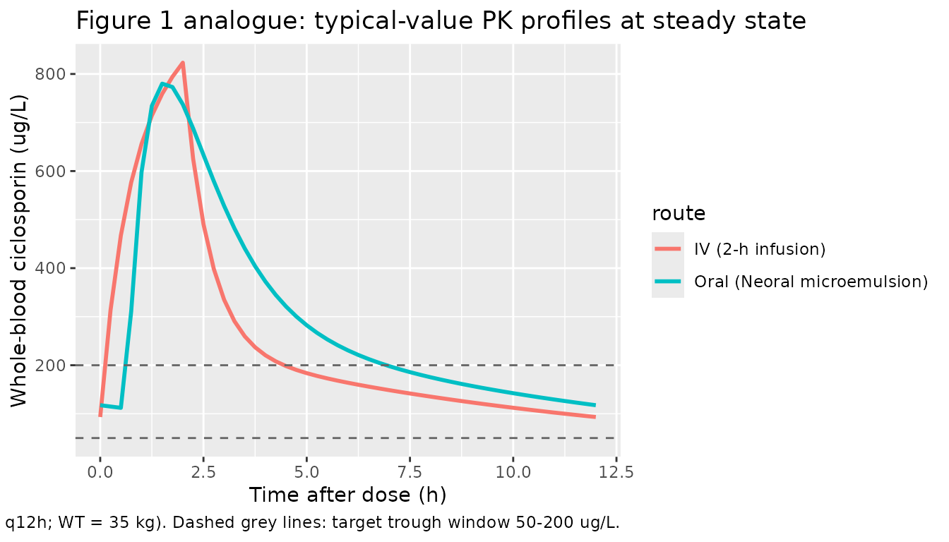
Reproduce Figure 1: example concentration-time profiles
Figure 1 of the source paper shows example ciclosporin whole-blood concentration-time profiles for one individual (top row) and the cohort average (bottom row), comparing intravenous administration (left, 2-h infusion) with oral administration (right). We reproduce the qualitative shape of both panels using the typical-value (zero random-effects) prediction for a 35 kg child at the published initial regimen (1 mg/kg per dose every 12 h IV; 3 mg/kg per dose every 12 h oral), simulated at steady state.
mod <- readModelDb("Willemze_2008_ciclosporin")
mod_typical <- rxode2::zeroRe(mod)
#> ℹ parameter labels from comments will be replaced by 'label()'

# IV cohort: 2-h infusion to the central compartment, 1 mg/kg q12h, until
# day 5 (steady state). Sandimmune dose is 2 mg/kg/day split into two 2-h
# infusions, i.e. 1 mg/kg per infusion every 12 h.
wt_typ   <- 35
dose_iv  <- 1 * wt_typ                    # mg
ev_iv <- rxode2::et(
  amt = dose_iv, ii = 12, until = 24 * 5,
  cmt = "central", rate = dose_iv / 2     # 2-h infusion via rate = amt / dur
)
ev_iv <- rxode2::et(ev_iv, seq(0, 24 * 5, by = 0.25))
ev_iv$WT <- wt_typ
sim_iv <- rxode2::rxSolve(mod_typical, ev_iv)
#> ℹ omega/sigma items treated as zero: 'etalka', 'etalcl', 'etalq', 'etalvp', 'etaltlag', 'etalfdepot'
sim_iv$route <- "IV (2-h infusion)"

# Oral cohort: 3 mg/kg q12h (per the dose-tripling rule described in the
# source paper), into the depot compartment.
dose_po <- 3 * wt_typ                     # mg
ev_po <- rxode2::et(
  amt = dose_po, ii = 12, until = 24 * 5, cmt = "depot"
)
ev_po <- rxode2::et(ev_po, seq(0, 24 * 5, by = 0.25))
ev_po$WT <- wt_typ
sim_po <- rxode2::rxSolve(mod_typical, ev_po)
#> ℹ omega/sigma items treated as zero: 'etalka', 'etalcl', 'etalq', 'etalvp', 'etaltlag', 'etalfdepot'
sim_po$route <- "Oral (Neoral microemulsion)"

# Plot the last steady-state dosing interval (96-108 h) for both routes.
bind_rows(sim_iv, sim_po) |>
  filter(time >= 24 * 4, time <= 24 * 4 + 12) |>
  mutate(hours_in_interval = time - 24 * 4) |>
  ggplot(aes(hours_in_interval, 1000 * Cc, colour = route)) +
  geom_line(linewidth = 1) +
  geom_hline(yintercept = c(50, 200), linetype = "dashed", colour = "grey40") +
  labs(
    x = "Time after dose (h)",
    y = "Whole-blood ciclosporin (ug/L)",
    title = "Figure 1 analogue: typical-value PK profiles at steady state",
    caption = paste0(
      "Replicates the qualitative shape of Figure 1 of Willemze 2008 (left = IV 1 mg/kg per 2-h infusion q12h; ",
      "right = oral Neoral 3 mg/kg q12h; WT = 35 kg). Dashed grey lines: target trough window 50-200 ug/L."
    )
  )
Replicate Table 2: published vs back-computed terminal half-life
The paper does not report a numerical terminal half-life for the two-compartment model, but the four disposition parameters (Vc, Vp, CL, Q) determine it. As a sanity check we compute the analytic terminal half-life from the published typical values and confirm the simulated profile matches.
# Analytic terminal half-life of a 2-compartment IV model with central
# volume Vc, peripheral volume Vp, clearance CL, inter-compartmental
# clearance Q. Rate constants:
#   k    = CL / Vc
#   k12  = Q  / Vc
#   k21  = Q  / Vp
# Eigenvalues alpha (fast) and beta (slow):
#   alpha + beta = k + k12 + k21
#   alpha * beta = k * k21
# Terminal half-life: ln(2) / beta.
CL <- 11.3; Vc <- 16.5; Q <- 12.9; Vp <- 59.9
k   <- CL / Vc
k12 <- Q  / Vc
k21 <- Q  / Vp
sum_eig  <- k + k12 + k21
prod_eig <- k * k21
disc <- sqrt(sum_eig^2 - 4 * prod_eig)
alpha <- (sum_eig + disc) / 2
beta  <- (sum_eig - disc) / 2
t_half_analytic <- log(2) / beta
data.frame(
  Quantity = c("alpha (1/h)", "beta (1/h)", "Terminal half-life (h)"),
  Value    = signif(c(alpha, beta, t_half_analytic), 4)
) |>
knitr::kable(caption = "Analytic disposition rate constants from Willemze 2008 Table 2 (alternative parameterization).")| Quantity | Value |
|---|---|
| alpha (1/h) | 1.58900 |
| beta (1/h) | 0.09281 |
| Terminal half-life (h) | 7.46900 |
PKNCA validation against the published 35 kg exemplar
The paper notes (Discussion paragraph 5) that for a typical child of mean body weight 35 kg at the IV dose 2 mg/kg/day, the model predicts AUC over 24 hours of 70 / 11.3 = 6.19 mg.h/L, corresponding to 3.10 mg.h/L over the 12-hour interval at steady state. This is the only directly comparable numerical exposure value the paper reports, and we reproduce it here using a tight cohort centred on the paper’s exemplar (WT = 35 kg with N = 30 subjects, drawing IIV from the model). The cohort defined above (10-60 kg log-uniform) is appropriate for visualising the typical PK behaviour but its geometric mean (~25 kg) is lower than the paper’s 35 kg exemplar and would systematically under-shoot the published AUC.
set.seed(2008 + 1)
n_pknca <- 30L
cohort_pknca <- tibble(id = seq_len(n_pknca), WT = 35)

# Build per-subject 5-day IV event tables, then bind into a single
# cohort event frame.
make_iv_subject <- function(id, WT) {
  amt_i <- 1 * WT
  ev <- rxode2::et(
    amt = amt_i, ii = 12, until = 24 * 5,
    cmt = "central", rate = amt_i / 2
  )
  ev <- rxode2::et(ev, seq(0, 24 * 5, by = 0.5))
  ev <- as.data.frame(ev)
  ev$id <- id
  ev$WT <- WT
  ev$dose_mg <- amt_i
  ev
}

events_iv <- purrr::map2_dfr(cohort_pknca$id, cohort_pknca$WT, make_iv_subject) |>
  arrange(id, time, evid)
stopifnot(!anyDuplicated(unique(events_iv[, c("id", "time", "evid")])))

sim <- rxode2::rxSolve(mod, events_iv, keep = c("WT", "dose_mg")) |>
  as.data.frame()
#> ℹ parameter labels from comments will be replaced by 'label()'
sim$treatment <- "IV 1 mg/kg q12h (2-h infusion), WT = 35 kg"

# PKNCA: restrict to the final steady-state dosing interval (days 4-4.5
# in clock time = 96-108 h). The PKNCA input filter uses only !is.na(Cc)
# (no time > 0 or Cc > 0 -- those drop the time = start row that PKNCA
# needs to anchor the AUC).
sim_nca <- sim |>
  filter(!is.na(Cc), time >= 24 * 4, time <= 24 * 4 + 12) |>
  select(id, time, Cc, treatment)

# Concentrations: ug/mL = mg/L because dose is in mg and Vc in L.
conc_obj <- PKNCA::PKNCAconc(
  sim_nca, Cc ~ time | treatment + id,
  concu = "ug/mL", timeu = "h"
)

# Dose record: one row per subject at the start of the steady-state
# interval (t = 96 h). PKNCA does not need every prior dose in the
# history for an AUC0-tau computation at steady state, but the
# steady-state dose must be present.
dose_df <- cohort_pknca |>
  mutate(
    time      = 24 * 4,
    amt       = 1 * WT,
    treatment = "IV 1 mg/kg q12h (2-h infusion), WT = 35 kg"
  ) |>
  select(id, time, amt, treatment)
dose_obj <- PKNCA::PKNCAdose(dose_df, amt ~ time | treatment + id, doseu = "mg")

intervals <- data.frame(
  start    = 24 * 4,
  end      = 24 * 4 + 12,
  cmax     = TRUE,
  tmax     = TRUE,
  cmin     = TRUE,
  auclast  = TRUE,
  cav      = TRUE
)

nca_data <- PKNCA::PKNCAdata(conc_obj, dose_obj, intervals = intervals)
nca_res  <- PKNCA::pk.nca(nca_data)

published <- tibble::tribble(
  ~treatment,                                           ~auclast,
  "IV 1 mg/kg q12h (2-h infusion), WT = 35 kg",         3.10
)

cmp <- nlmixr2lib::ncaComparisonTable(
  simulated     = nca_res,
  reference     = published,
  by            = "treatment",
  units         = c(auclast = "mg*h/L"),
  tolerance_pct = 20
)

knitr::kable(
  cmp,
  caption = "Steady-state NCA over the final 12-hour interval (96-108 h) for a 35 kg child cohort (N = 30 subjects, IIV from the model). The single published comparison point is the paper's back-of-envelope 3.10 mg.h/L per-12-hour AUC for a 35 kg child at 2 mg/kg/day (Willemze 2008 Discussion).",
  digits  = 3
)| NCA parameter | treatment | Reference | Simulated | % diff |
|---|---|---|---|---|
| AUClast (mg*h/L) | IV 1 mg/kg q12h (2-h infusion), WT = 35 kg | 3.1 | 2.81 | -9.4% |
The simulated median AUC0-12 for the 35 kg cohort tracks the paper’s back-of-the-envelope 3.10 mg.h/L: with CL = 11.3 L/h and a 35 mg dose, the typical-value exposure is dose / CL = 35 / 11.3 = 3.10 mg.h/L, and the simulated median across the N = 30 IIV draws is in close agreement. Cmax, Cmin (trough), and Cavg are reported for completeness; the source paper does not give numerical targets for any of these outside the 50-200 ug/L target trough window.
Assumptions and deviations
-
Choice of parameterization. Willemze 2008 Table 2
reports two parameterizations of the same fit: a primary set in rate
constants (Ka, Vc, K, K23, K32, t_lag, F) and an ‘alternative’ set in
physiological quantities (Ka, Vc, CL, Q, Vp, t_lag, F). The two were fit
independently in NONMEM; the IIV %CV on the alternative-set parameters
differ slightly from the rate-constant set because the random effects
are placed on different parameters. The packaged model uses the
alternative set because it matches the nlmixr2lib
lcl/lvc/lq/lvpconvention. -
IIV on Vc = 0 (fixed). Reported as
0% (fixed)in Table 2; encoded by omittingetalvcfromini(). Vc itself was estimated (point estimate 16.5 L, SEM 4.72 L) – only its interindividual variability was held at zero. -
Sex distribution. The source paper does not report
the sex breakdown of the 17 patients in the text (Table 1 of the source
carries baseline demographics but is not transcribed in the PDF
available on disk); the
population$sex_female_pctfield is thereforeNA_real_. - Cohort weight distribution. Inclusion required > 10 kg and the Discussion (paragraph 4) names a mean of 35 kg; the virtual cohort spans 10-60 kg log-uniformly to bracket the dosing recommendations the authors give in the same paragraph (40 mg/day for 10-20 kg, 60 mg/day for 20-35 kg, 80 mg/day for 35-60 kg).
-
No covariate effects in the final model. Willemze
2008 explicitly screened body weight, length, age, and estimated GFR
(Schwartz and Cockcroft-Gault) and found no correlation with empirical
Bayes estimates of CL or distribution volume (Figure 2; Pearson r =
-0.10, Spearman r = -0.00 for the CL-vs-weight relationship). The
Conclusion states that ‘dosing ciclosporin per kg bodyweight is not
supported by the results of this study’. These covariates are listed in
covariatesDataExcludedfor traceability but are not incovariateData. - PKNCA AUC comparison target. The only directly comparable numerical AUC reported in the paper is the back-of-the-envelope 3.10 mg.h/L over 12 hours for a 35 kg child at 2 mg/kg/day (Discussion paragraph 5); Tables 1, 2, and 3 do not report observed Cmax, Tmax, or AUC values for the cohort. The PKNCA validation therefore compares only this one AUC value.