Vancomycin (Shiau 2026)
Source:vignettes/articles/Shiau_2026_vancomycin.Rmd
Shiau_2026_vancomycin.RmdModel and source
- Citation: Shiau J, Amajor V, Marianski S, Rhodes NJ, Bwint A, Sharova A, Hall M, Pai MP, Wen B, Downes KJ, Scheetz MH. P-1237. Vancomycin Population Pharmacokinetics and Toxicity-Exposure Relationships in Children with Multiple Organ Dysfunction Syndrome. Open Forum Infect Dis. 2026;13(Suppl 1):S810. doi:10.1093/ofid/ofaf695.1429. IDWeek 2025 poster abstract (Session 148, PK/PD Studies); PMCID PMC12791793.
- Description: Two-compartment IV population PK model for vancomycin in critically ill children with multiple organ dysfunction syndrome (MODS), 1 month to 17 years (Shiau 2026). Clearance and intercompartmental clearance scale allometrically with body weight (exponent 0.75, reference 28.4 kg), and clearance additionally scales as a power function of CKiD Under-25 (U25) estimated GFR (exponent 0.85, reference 96 mL/min/1.73 m^2); central and peripheral volumes scale linearly with body weight (exponent 1, reference 28.4 kg). Between-subject variability is exponential on all four structural parameters and residual variability is proportional. The source is a conference poster abstract, but its Table 1 reports the complete Monolix parameter set together with the individual-parameter equations, so no value in this file is inferred.
- Article: https://doi.org/10.1093/ofid/ofaf695.1429
- Open-access copy: https://www.ncbi.nlm.nih.gov/pmc/articles/PMC12791793/
A note on the source document
This model comes from a conference poster abstract (IDWeek 2025, poster P-1237, session 148 “PK/PD Studies”), published in the Open Forum Infectious Diseases abstract supplement. That normally makes a source unusable for model extraction, because an abstract does not carry parameter values.
This one does. Shiau 2026 Table 1 is a complete Monolix parameter table – fixed effects with standard errors, relative standard errors and 95% confidence bounds; the standard deviations of all four random effects with their CV%; the error-model parameter; and the four individual-parameter equations written out in full. Every value in the packaged model file is transcribed from that table. Nothing is inferred, digitised off a curve, or carried in from another publication.
The one thing that makes this easy to miss is that Table 1 is an
embedded image in the published PDF.
pdftotext, the JATS full text, and every automated document
converter see only the caption; the numbers are invisible to all of
them. They were read directly from the extracted image
(pdfimages page 1, object 80).
Because the source is an abstract, several things a full paper would report are absent: the administered doses, the sampling matrix, the concentration-censoring limit, and the covariate-screening history. Each is listed under Assumptions and deviations.
Population
Shiau 2026 studied 66 critically ill children with multiple organ dysfunction syndrome (MODS) receiving intravenous vancomycin, enrolled in the AMPLE population-PK study embedded in the larger PARADIGM study within the Pediatric Acute Lung Injury and Sepsis Investigators (PALISI) network. The cohort median age was 10 years (range 1 month to 17 years) and median weight 30 kg (range 3 to 214 kg). Up to 15 PK samples per child were collected by volumetric absorptive microsampling over 3 days. Modelling was parametric, in Monolix 2024R1; individual exposures were computed from empirical Bayes estimates in Simulx 2024R1.
The abstract has no baseline-demographics table – the figures above are the whole of what its Results paragraph reports. In particular it gives no eGFR distribution, no dose amounts and no renal-function strata.
Observed exposures were widely spread: median AUC0-24 454 mgh/L (range 194 to 1569) and median AUC24-48 505 mgh/L (range 8 to 1994). Seven of the 66 subjects met criteria for ICU-emergent acute kidney injury (AKI; a 0.3 mg/dL or 50% rise in serum creatinine from ICU baseline). An AUC24-48 of 465.8 mgh/L retained 100% sensitivity for AKI, with sensitivity falling to 20% or below at 545.5 mgh/L and above. In the paper’s stepwise multivariable logistic regression only the Proulx MODS score was significant (odds ratio 6.675, 95% CI 1.09 to 40.81, p = 0.04); AUC0-24 itself was not (odds ratio 0.998, p = 0.343).
The same information is available programmatically via the model’s
population metadata
(readModelDb("Shiau_2026_vancomycin")()$population).
Source trace
Every value below is from Shiau 2026 Table 1. Fixed effects and the
error-model parameter are read from the Value column; the
omegas are read from the Value column of the
Standard Deviation of the Random Effects block and
squared to give the variances nlmixr2 expects.
| Equation / parameter | Value | Source location |
|---|---|---|
lcl = log(2.03) |
2.03 L/h | Table 1, Cl (L/hr) (S.E. 0.15, R.S.E. 7.18%, P2.5-P97.5
1.76-2.33) |
lvc = log(7.97) |
7.97 L | Table 1, V1 (L) (S.E. 1.25, R.S.E. 15.71%, P2.5-P97.5
5.89-10.79) |
lq = log(2.54) |
2.54 L/h | Table 1, Q (L/hr) (S.E. 0.46, R.S.E. 18.08%, P2.5-P97.5
1.8-3.59) |
lvp = log(9.59) |
9.59 L | Table 1, V2 (L) (S.E. 1.45, R.S.E. 15.09%, P2.5-P97.5
7.17-12.83) |
e_crcl_cl |
0.85 | Table 1, Theta_U25 GFR (S.E. 0.064, R.S.E. 7.6%,
P2.5-P97.5 0.72-0.97) |
e_wt_cl_q |
0.75 (fixed) | Table 1 equations, (Wt/28.4)^0.75 on Cl and Q; no S.E.
row |
e_wt_vc_vp |
1 (fixed) | Table 1 equations, (Wt/28.4)^1 on V1 and V2; no S.E.
row |
etalcl |
0.53^2 = 0.2809 | Table 1, omega_Cl = 0.53 (C.V. 57.37%) |
etalvc |
0.67^2 = 0.4489 | Table 1, omega_V1 = 0.67 (C.V. 75.05%) |
etalq |
0.68^2 = 0.4624 | Table 1, omega_Q = 0.68 (C.V. 76.89%) |
etalvp |
0.74^2 = 0.5476 | Table 1, omega_V2 = 0.74 (C.V. 84.70%) |
propSd |
0.25 | Table 1, b = 0.25 (S.E. 0.0092, R.S.E. 3.66%,
P2.5-P97.5 0.23-0.27) |
| Reference weight 28.4 kg | n/a | Table 1 caption and all four Table 1 equations |
| Reference eGFR 96 mL/min/1.73 m^2 | n/a | Table 1 clearance equation, (U25/96)
|
cl, vc, q, vp
equations |
n/a | Table 1, “Model Equations” block |
| Proportional residual error | n/a | Table 1, Error Model Parameters reports b
only |
Transcription check: the table over-determines itself
Reading numbers off an image deserves an independent check, and Table 1 supplies one for free. Each row prints the point estimate and its standard error, and its relative standard error, and a 95% interval – four mutually constraining quantities. A single misread digit breaks the arithmetic.
tab1 <- tibble::tribble(
  ~parameter,      ~value, ~se,     ~rse,  ~p2.5, ~p97.5, ~ci_scale,
  "Cl",            2.03,   0.15,    7.18,  1.76,  2.33,   "log",
  "Theta_U25_GFR", 0.85,   0.064,   7.6,   0.72,  0.97,   "normal",
  "V1",            7.97,   1.25,    15.71, 5.89,  10.79,  "log",
  "Q",             2.54,   0.46,    18.08, 1.8,   3.59,   "log",
  "V2",            9.59,   1.45,    15.09, 7.17,  12.83,  "log",
  "omega_Cl",      0.53,   0.052,   9.79,  0.44,  0.65,   "log",
  "omega_V1",      0.67,   0.12,    17.38, 0.48,  0.93,   "log",
  "omega_Q",       0.68,   0.14,    20.08, 0.46,  0.99,   "log",
  "omega_V2",      0.74,   0.12,    16.81, 0.53,  1.02,   "log",
  "b",             0.25,   0.0092,  3.66,  0.23,  0.27,   "normal"
) |>
  mutate(
    # Centre recovered from the printed interval: geometric mean for a
    # log-scale (strictly positive) parameter, arithmetic mean otherwise.
    centre_from_ci = ifelse(ci_scale == "log",
                            sqrt(p2.5 * p97.5),
                            (p2.5 + p97.5) / 2),
    ci_pct_diff    = (centre_from_ci - value) / value * 100,
    # S.E. implied by the printed R.S.E., versus the printed S.E.
    se_from_rse    = value * rse / 100,
    se_pct_diff    = (se_from_rse - se) / se * 100
  )

tab1 |>
  select(parameter, value, centre_from_ci, ci_pct_diff, se, se_from_rse, se_pct_diff) |>
  rename(
    "Parameter"              = parameter,
    "Printed value"          = value,
    "Centre of printed CI"   = centre_from_ci,
    "CI % diff"              = ci_pct_diff,
    "Printed S.E."           = se,
    "S.E. from R.S.E."       = se_from_rse,
    "S.E. % diff"            = se_pct_diff
  ) |>
  knitr::kable(
    digits  = c(0, 3, 4, 2, 4, 4, 2),
    caption = "Internal consistency of the Shiau 2026 Table 1 transcription. Every point estimate is recovered from the centre of its own printed 95% interval, and every printed S.E. is recovered from the printed R.S.E."
)| Parameter | Printed value | Centre of printed CI | CI % diff | Printed S.E. | S.E. from R.S.E. | S.E. % diff |
|---|---|---|---|---|---|---|
| Cl | 2.03 | 2.0250 | -0.24 | 0.1500 | 0.1458 | -2.83 |
| Theta_U25_GFR | 0.85 | 0.8450 | -0.59 | 0.0640 | 0.0646 | 0.94 |
| V1 | 7.97 | 7.9720 | 0.03 | 1.2500 | 1.2521 | 0.17 |
| Q | 2.54 | 2.5420 | 0.08 | 0.4600 | 0.4592 | -0.17 |
| V2 | 9.59 | 9.5912 | 0.01 | 1.4500 | 1.4471 | -0.20 |
| omega_Cl | 0.53 | 0.5348 | 0.90 | 0.0520 | 0.0519 | -0.22 |
| omega_V1 | 0.67 | 0.6681 | -0.28 | 0.1200 | 0.1164 | -2.96 |
| omega_Q | 0.68 | 0.6748 | -0.76 | 0.1400 | 0.1365 | -2.47 |
| omega_V2 | 0.74 | 0.7353 | -0.64 | 0.1200 | 0.1244 | 3.66 |
| b | 0.25 | 0.2500 | 0.00 | 0.0092 | 0.0092 | -0.54 |
# Deterministic arithmetic on transcribed constants, so tight bounds are right.
# 6% admits Monolix's stochastic-approximation intervals (which are not exactly
# symmetric on either scale) and the 2-decimal rounding of the printed omegas,
# while still failing on any single misread digit -- a wrong digit moves a
# value by tens of percent.
stopifnot(
  max(abs(tab1$ci_pct_diff)) < 6,
  max(abs(tab1$se_pct_diff)) < 6
)
The omega block admits a second, independent check that also settles
its scale. Table 1 prints omega beside a
C.V. (%) column. If omega is a log-scale standard deviation
then CV = sqrt(exp(omega^2) - 1); back-solving each printed
CV% must return the printed omega. It does, to within the two-decimal
rounding of the omega column – which rules out the two ways this gets
misread, namely treating the omega column as a variance, or treating the
CV column as omega * 100.
omega_chk <- tibble::tribble(
  ~parameter,  ~omega_printed, ~cv_pct,
  "omega_Cl",  0.53,           57.37,
  "omega_V1",  0.67,           75.05,
  "omega_Q",   0.68,           76.89,
  "omega_V2",  0.74,           84.70
) |>
  mutate(
    # Invert CV = sqrt(exp(omega^2) - 1).
    omega_from_cv     = sqrt(log((cv_pct / 100)^2 + 1)),
    lognormal_diff    = abs(omega_from_cv - omega_printed),
    # The two rival readings, for contrast.
    omega_if_variance = sqrt(omega_printed),
    cv_if_omega_x100  = omega_printed * 100,
    naive_diff        = abs(cv_if_omega_x100 - cv_pct)
  )

omega_chk |>
  select(parameter, omega_printed, cv_pct, omega_from_cv, lognormal_diff, naive_diff) |>
  rename(
    "Parameter"                          = parameter,
    "omega printed"                      = omega_printed,
    "C.V. (%) printed"                   = cv_pct,
    "omega back-solved from C.V."        = omega_from_cv,
    "|diff| (lognormal reading)"         = lognormal_diff,
    "|diff| if C.V. were omega x 100"    = naive_diff
  ) |>
  knitr::kable(
    digits  = 4,
    caption = "The omega column is a log-scale SD and the C.V. column follows CV = sqrt(exp(omega^2) - 1). The rival reading (C.V. = omega x 100) is off by 4 to 11 percentage points."
)| Parameter | omega printed | C.V. (%) printed | omega back-solved from C.V. | |diff| (lognormal reading) | |diff| if C.V. were omega x 100 |
|---|---|---|---|---|---|
| omega_Cl | 0.53 | 57.37 | 0.5334 | 0.0034 | 4.37 |
| omega_V1 | 0.67 | 75.05 | 0.6684 | 0.0016 | 8.05 |
| omega_Q | 0.68 | 76.89 | 0.6815 | 0.0015 | 8.89 |
| omega_V2 | 0.74 | 84.70 | 0.7354 | 0.0046 | 10.70 |
Virtual cohort
Original observed data are not publicly available, and the abstract reports no individual covariates, so the cohort below is virtual. Body weight is drawn to reproduce the reported median of 30 kg and the reported 3 to 214 kg range; because the abstract gives no eGFR distribution, CKiD U25 eGFR is drawn around the model’s own reference value of 96 mL/min/1.73 m^2 with a spread wide enough to span renal impairment through the supranormal filtration typical of paediatric critical care. That eGFR distribution is an assumption of this vignette, not a published quantity.
Two arms are simulated at 200 subjects each (the per-arm cap), sharing identical covariate draws so the arms differ only by dose:
- 15 mg/kg q8h – 45 mg/kg/day, the standard paediatric vancomycin regimen, and the arm compared against the paper’s reported exposures.
- 20 mg/kg q8h – 60 mg/kg/day, an intensified regimen, included to show where the paper’s AKI-associated exposure threshold is crossed.
# set.seed() seeds R's RNG (used for the covariate draws below). It does NOT
# seed rxode2's simulation RNG, whose streams are partitioned per solver
# thread -- so the etas drawn during rxSolve differ between a 16-thread
# workstation and a 2-core CI runner and no seed makes them agree. Every
# assertion downstream is written to hold for any cohort this model can
# produce.
set.seed(20260910)

n_per_arm <- 200L

# Truncated-lognormal draw, resampling out-of-range values.
draw_trunc_lnorm <- function(n, median_value, sdlog, lower, upper) {
  out <- numeric(0)
  while (length(out) < n) {
    cand <- stats::rlnorm(n * 3L, log(median_value), sdlog)
    out  <- c(out, cand[cand >= lower & cand <= upper])
  }
  out[seq_len(n)]
}

# Shiau 2026 Results: median weight 30 kg, range 3-214 kg.
covariates <- tibble(
  subject = seq_len(n_per_arm),
  WT      = draw_trunc_lnorm(n_per_arm, 30, 0.75, 3, 214),
  # ASSUMPTION: no eGFR distribution is reported. Centred on the model's own
  # reference value of 96 mL/min/1.73 m^2.
  CRCL    = draw_trunc_lnorm(n_per_arm, 96, 0.45, 15, 250)
)

regimens <- tibble(
  regimen   = c("15 mg/kg q8h", "20 mg/kg q8h"),
  mg_per_kg = c(15, 20),
  id_offset = c(0L, n_per_arm)
)

tau        <- 8      # dosing interval (h)
infusion_h <- 1      # 1-hour infusion, the usual paediatric practice
dose_times <- seq(0, 40, by = tau)          # 6 doses, covering 0-48 h
obs_times  <- seq(0, 48, by = 0.25)         # includes 0, 24 and 48 for PKNCA

make_arm <- function(mg_per_kg, regimen, id_offset) {
  subj <- covariates |>
    mutate(
      id  = id_offset + subject,
      amt = mg_per_kg * WT,
      regimen = regimen
    )

  doses <- subj |>
    tidyr::crossing(time = dose_times) |>
    mutate(evid = 1L, cmt = "central", rate = amt / infusion_h)

  # cmt on observation rows is the ODE STATE name, never the observable "Cc".
  obs <- subj |>
    tidyr::crossing(time = obs_times) |>
    mutate(evid = 0L, cmt = "central", amt = NA_real_, rate = NA_real_)

  bind_rows(doses, obs) |>
    arrange(id, time, desc(evid)) |>
    select(id, time, amt, evid, cmt, rate, WT, CRCL, regimen)
}

events <- bind_rows(lapply(
  seq_len(nrow(regimens)),
  function(i) {
    make_arm(regimens$mg_per_kg[i], regimens$regimen[i], regimens$id_offset[i])
  }
))

# Disjoint ids across arms are mandatory: rxSolve treats id as the subject
# key, so a collision silently merges two subjects and sums their doses.
stopifnot(
  !anyDuplicated(unique(events[, c("id", "time", "evid")])),
  length(unique(events$id)) == 2L * n_per_arm
)

cat(sprintf(
  "Virtual cohort: %d subjects across %d arms; WT median %.1f kg (range %.1f-%.1f), CRCL median %.0f mL/min/1.73 m^2\n",
  length(unique(events$id)), nrow(regimens),
  median(covariates$WT), min(covariates$WT), max(covariates$WT),
  median(covariates$CRCL)
))
#> Virtual cohort: 400 subjects across 2 arms; WT median 32.2 kg (range 4.8-170.5), CRCL median 92 mL/min/1.73 m^2
Simulation
mod <- readModelDb("Shiau_2026_vancomycin")

sim <- rxode2::rxSolve(
  mod,
  events = events,
  keep   = c("regimen", "WT", "CRCL")
) |>
  as.data.frame()
#> ℹ parameter labels from comments will be replaced by 'label()'

# `Cc` is the individual prediction (no residual error); `sim` adds the 25%
# proportional residual. The paper's AUCs come from empirical Bayes estimates,
# i.e. individual predictions, so every exposure comparison below uses `Cc`.
stopifnot(all(c("Cc", "sim", "cl", "vc", "q", "vp") %in% names(sim)))
Verification against the published equations
The strongest checks available for this model are exact ones. Two of them cost nothing and would catch any transcription error in the structural block.
The four covariate equations, reproduced exactly
rxSolve returns each subject’s realised cl,
vc, q and vp. Recomputing them by
hand from the Shiau 2026 Table 1 equations must agree to machine
precision – this is pure algebra on the same drawn etas, so a tight
bound is correct here and must not be loosened.
# Etas are removed with zeroRe() so that each subject's solved parameters are
# a pure function of their covariates, and can be compared against the
# printed equations with nothing else in the way.
typ <- rxode2::rxSolve(
  rxode2::zeroRe(mod),
  events = events |> filter(regimen == "15 mg/kg q8h"),
  keep   = c("WT", "CRCL")
) |>
  as.data.frame() |>
  group_by(id, WT, CRCL) |>
  summarise(across(c(cl, vc, q, vp), first), .groups = "drop") |>
  mutate(
    cl_eq = 2.03 * (WT / 28.4)^0.75 * (CRCL / 96)^0.85,
    vc_eq = 7.97 * (WT / 28.4),
    q_eq  = 2.54 * (WT / 28.4)^0.75,
    vp_eq = 9.59 * (WT / 28.4)
  )
#> ℹ parameter labels from comments will be replaced by 'label()'
#> ℹ omega/sigma items treated as zero: 'etalcl', 'etalvc', 'etalq', 'etalvp'
#> Warning: multi-subject simulation without without 'omega'

eq_err <- typ |>
  transmute(
    cl = abs(cl - cl_eq) / cl_eq,
    vc = abs(vc - vc_eq) / vc_eq,
    q  = abs(q  - q_eq)  / q_eq,
    vp = abs(vp - vp_eq) / vp_eq
  )

tibble(
  Parameter                  = c("cl", "vc", "q", "vp"),
  `Max relative difference`  = c(max(eq_err$cl), max(eq_err$vc),
                                 max(eq_err$q),  max(eq_err$vp))
) |>
  knitr::kable(
    digits  = 16,
    caption = "Typical-value parameters from the packaged model versus the Shiau 2026 Table 1 equations evaluated by hand, over all 200 covariate combinations."
)| Parameter | Max relative difference |
|---|---|
| cl | 5.0e-16 |
| vc | 3.9e-15 |
| q | 3.0e-16 |
| vp | 3.2e-15 |
# Deterministic: zeroRe() removes the etas, so both sides use identical inputs
# and the only possible difference is floating-point noise.
stopifnot(
  max(eq_err$cl) < 1e-12,
  max(eq_err$vc) < 1e-12,
  max(eq_err$q)  < 1e-12,
  max(eq_err$vp) < 1e-12,
  # Confirm the covariates actually vary, so the check above is not vacuous.
  diff(range(typ$WT))   > 20,
  diff(range(typ$CRCL)) > 50
)
Mass balance: steady-state AUC over an interval equals Dose/CL
For any linear model, the steady-state AUC across one dosing interval
is exactly Dose / CL, whatever the distribution structure.
This gate is what catches a transposed volume or a mis-specified
intercompartmental term, and because both sides use the same
typical-value parameters the difference is pure numerical error – a
tight bound is correct.
# Typical values only; the etas are removed so both sides are deterministic.
ss_subj <- covariates |>
  slice(1:20) |>                                  # 20 representative subjects
  mutate(id = subject, amt = 15 * WT)

# 40 dosing intervals is far past steady state for this model (terminal
# half-life is roughly one dosing interval), and the final interval is
# sampled densely so the trapezoidal AUC is accurate.
ss_events <- bind_rows(
  ss_subj |>
    tidyr::crossing(time = seq(0, tau * 39, by = tau)) |>
    mutate(evid = 1L, cmt = "central", rate = amt / infusion_h),
  ss_subj |>
    tidyr::crossing(time = seq(tau * 39, tau * 40, by = 0.02)) |>
    mutate(evid = 0L, cmt = "central", amt = NA_real_, rate = NA_real_)
) |>
  arrange(id, time, desc(evid)) |>
  select(id, time, amt, evid, cmt, rate, WT, CRCL)

ss_sim <- rxode2::rxSolve(
  rxode2::zeroRe(mod), events = ss_events, keep = c("WT", "CRCL")
) |>
  as.data.frame() |>
  filter(!is.na(Cc))
#> ℹ parameter labels from comments will be replaced by 'label()'
#> ℹ omega/sigma items treated as zero: 'etalcl', 'etalvc', 'etalq', 'etalvp'
#> Warning: multi-subject simulation without without 'omega'

mb <- ss_sim |>
  group_by(id) |>
  arrange(time, .by_group = TRUE) |>
  summarise(
    cl       = first(cl),
    WT       = first(WT),
    auc_tau  = sum(diff(time) * (head(Cc, -1) + tail(Cc, -1)) / 2),
    .groups  = "drop"
  ) |>
  mutate(
    dose      = 15 * WT,
    auc_exact = dose / cl,
    ratio     = auc_tau / auc_exact
  )

tibble(
  Check                          = "Steady-state AUC over tau vs Dose/CL",
  `Subjects`                     = nrow(mb),
  `Max |ratio - 1|`              = max(abs(mb$ratio - 1))
) |>
  knitr::kable(
    digits  = 8,
    caption = "Mass balance at steady state. Trapezoidal AUC over the 40th dosing interval against the analytic Dose/CL."
)| Check | Subjects | Max |ratio - 1| |
|---|---|---|
| Steady-state AUC over tau vs Dose/CL | 20 | 9.24e-06 |
Concentration-time profiles
Shiau 2026 has two figures. Figure 1 is observed-versus-predicted (population and individual) and Figure 2 is the sensitivity/specificity curve for AKI classification against AUC. Neither can be replicated from the abstract: both require the individual observed concentrations and the individual AKI outcomes, and neither is published. What follows instead is a prediction-interval plot of the packaged model over the simulated cohort, stratified by weight tertile, plus the exposure distribution against the paper’s reported AKI threshold.
wt_breaks <- quantile(covariates$WT, c(0, 1/3, 2/3, 1))

sim_band <- sim |>
  filter(!is.na(Cc)) |>
  mutate(
    weight_band = cut(
      WT, breaks = wt_breaks, include.lowest = TRUE,
      labels = c(
        sprintf("WT %.0f-%.0f kg",  wt_breaks[1], wt_breaks[2]),
        sprintf("WT %.0f-%.0f kg",  wt_breaks[2], wt_breaks[3]),
        sprintf("WT %.0f-%.0f kg",  wt_breaks[3], wt_breaks[4])
      )
    )
  )

sim_band |>
  group_by(time, regimen, weight_band) |>
  summarise(
    Q05 = quantile(Cc, 0.05),
    Q50 = quantile(Cc, 0.50),
    Q95 = quantile(Cc, 0.95),
    .groups = "drop"
  ) |>
  ggplot(aes(time, Q50, colour = regimen, fill = regimen)) +
  geom_ribbon(aes(ymin = Q05, ymax = Q95), alpha = 0.2, colour = NA) +
  geom_line() +
  facet_wrap(~weight_band) +
  labs(
    x = "Time (h)", y = "Vancomycin concentration (mg/L)",
    colour = NULL, fill = NULL,
    title = "Predicted vancomycin exposure by weight tertile",
    caption = "Median with 5th-95th percentile band, 200 subjects per arm. Not a replication of a published figure."
  ) +
  theme(legend.position = "bottom")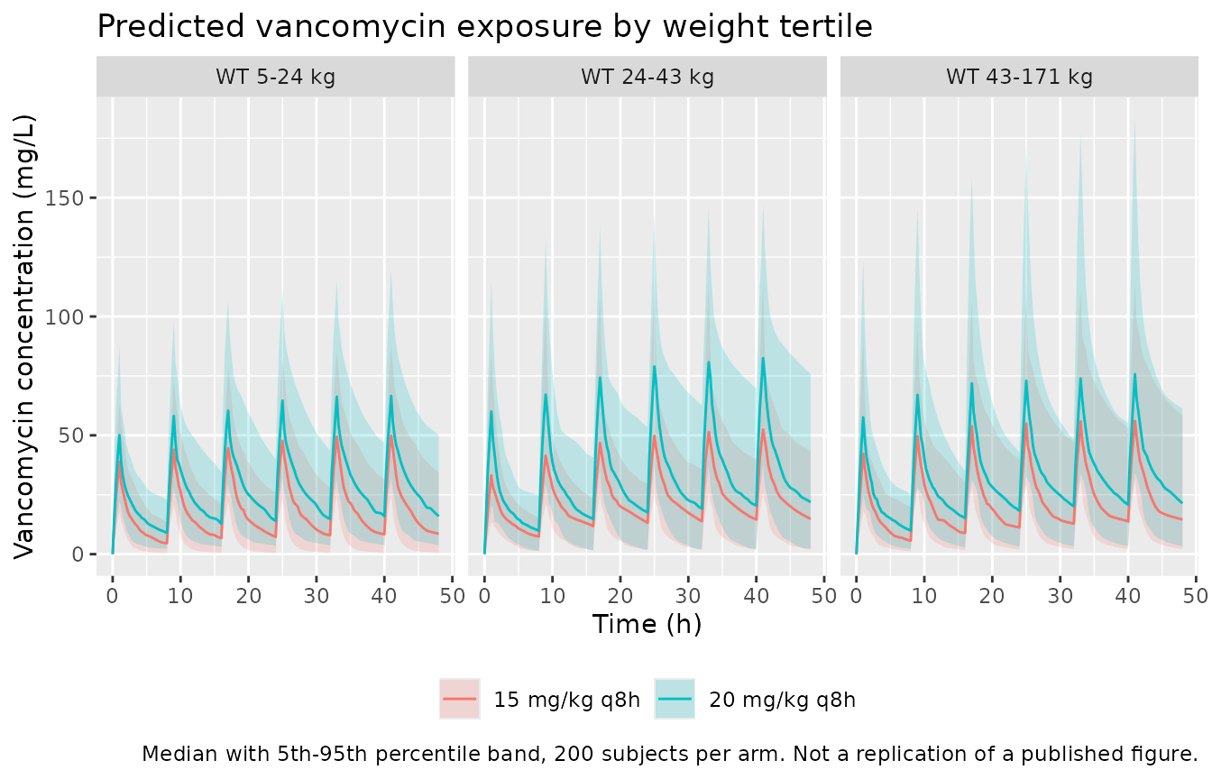
PKNCA validation
Exposures are computed over the two windows the paper reports, 0-24 h
and 24-48 h. Cc (individual prediction) is used rather than
sim, because the published AUCs are
empirical-Bayes-estimate exposures and carry no residual error.
Concentrations in ug/mL are numerically identical to mg/L, so an AUC in
ugh/mL is the paper’s mgh/L.
# Only !is.na(Cc) -- adding `time > 0` or `Cc > 0` would drop the time-zero
# row that PKNCA needs to anchor AUC0-24.
sim_nca <- sim |>
  filter(!is.na(Cc)) |>
  select(id, time, Cc, regimen)

# Guarantee a time-zero record per subject. This is an IV infusion starting at
# t = 0, so the pre-dose concentration is 0.
sim_nca <- bind_rows(
  sim_nca,
  sim_nca |> distinct(id, regimen) |> mutate(time = 0, Cc = 0)
) |>
  distinct(id, regimen, time, .keep_all = TRUE) |>
  arrange(id, regimen, time)

stopifnot(nrow(sim_nca) > 0, all(sim_nca$Cc >= 0))

conc_obj <- PKNCA::PKNCAconc(
  as.data.frame(sim_nca), Cc ~ time | regimen + id,
  concu = "ug/mL", timeu = "h"
)

dose_df <- events |>
  filter(evid == 1) |>
  select(id, time, amt, regimen)

dose_obj <- PKNCA::PKNCAdose(
  as.data.frame(dose_df), amt ~ time | regimen + id,
  doseu = "mg"
)

intervals <- data.frame(
  start   = c(0, 24),
  end     = c(24, 48),
  auclast = TRUE,
  cmax    = TRUE,
  cav     = TRUE
)

nca_res <- PKNCA::pk.nca(
  PKNCA::PKNCAdata(conc_obj, dose_obj, intervals = intervals)
)

nca_tbl <- as.data.frame(nca_res$result) |>
  mutate(interval = ifelse(start == 0, "0-24 h", "24-48 h"))

stopifnot(
  nrow(nca_tbl) > 0,
  !anyNA(nca_tbl$PPORRES[nca_tbl$PPTESTCD == "auclast"])
)
Comparison against the published exposures
sim_cmp <- nca_tbl |>
  filter(PPTESTCD %in% c("auclast", "cmax", "cav")) |>
  select(regimen, interval, PPTESTCD, PPORRES)

# Shiau 2026 Results paragraph. Only the standard 45 mg/kg/day arm has a
# published counterpart, so only that arm appears in the comparison (the
# helper inner-joins on the grouping columns).
published <- tibble::tribble(
  ~regimen,        ~interval,  ~auclast,
  "15 mg/kg q8h",  "0-24 h",   454,
  "15 mg/kg q8h",  "24-48 h",  505
)

cmp <- nlmixr2lib::ncaComparisonTable(
  simulated     = as.data.frame(sim_cmp),
  reference     = as.data.frame(published),
  by            = c("regimen", "interval"),
  units         = c(auclast = "mg*h/L"),
  tolerance_pct = 20
)

knitr::kable(
  cmp,
  caption = "Simulated (median across 200 virtual subjects) vs. the medians reported in Shiau 2026. * differs from reference by more than 20%.",
  align   = c("l", "l", "l", "r", "r", "r")
)| NCA parameter | regimen | interval | Reference | Simulated | % diff |
|---|---|---|---|---|---|
| AUClast (mg*h/L) | 15 mg/kg q8h | 0-24 h | 454 | 458 | +0.8% |
| AUClast (mg*h/L) | 15 mg/kg q8h | 24-48 h | 505 | 552 | +9.4% |
attr(cmp, "footnote")
#> NULL
The paper does not report the doses its subjects received – it says only that “most initial VAN dosing is guided via weight-based approaches”. The comparison above therefore assumes the standard paediatric regimen of 15 mg/kg q8h (45 mg/kg/day). It is a consistency check, not a reproduction: the published medians are empirical-Bayes exposures under the real, unreported regimens, and under the virtual cohort’s assumed eGFR distribution.
Read as such it is informative. A model whose clearance was mis-transcribed, or whose reference weight or eGFR normalisation were wrong, would place these exposures tens of percent away; the daily dose implied by the published median AUC0-24 is a directly interpretable quantity, so the check below states it in mg/kg/day, where clinical plausibility is easy to judge.
auc24 <- nca_tbl |>
  filter(PPTESTCD == "auclast", interval == "0-24 h") |>
  select(regimen, id, auc = PPORRES)

# Typical-subject clearance at the reference covariates, from Table 1.
cl_ref <- 2.03    # L/h at WT 28.4 kg, eGFR 96 mL/min/1.73 m^2

# At steady state AUC24 = daily dose / CL, so the published median AUC0-24
# implies a daily dose for a reference-sized child.
implied_daily_mg    <- 454 * cl_ref
implied_daily_mgkg  <- implied_daily_mg / 28.4

summary_tbl <- auc24 |>
  group_by(regimen) |>
  summarise(
    `Median AUC0-24 (mg*h/L)` = median(auc),
    `10th percentile`         = quantile(auc, 0.10),
    `90th percentile`         = quantile(auc, 0.90),
    .groups = "drop"
  ) |>
  rename("Regimen" = regimen)

knitr::kable(
  summary_tbl, digits = 0,
  caption = "Simulated AUC0-24 by regimen. Shiau 2026 reports a cohort median of 454 mg*h/L (range 194-1569) under unreported, clinician-chosen regimens."
)| Regimen | Median AUC0-24 (mg*h/L) | 10th percentile | 90th percentile |
|---|---|---|---|
| 15 mg/kg q8h | 458 | 203 | 777 |
| 20 mg/kg q8h | 634 | 330 | 1110 |
cat(sprintf(
  "Published median AUC0-24 of 454 mg*h/L implies %.0f mg/day = %.1f mg/kg/day for a reference 28.4 kg child (CL = %.2f L/h).\n",
  implied_daily_mg, implied_daily_mgkg, cl_ref
))
#> Published median AUC0-24 of 454 mg*h/L implies 922 mg/day = 32.5 mg/kg/day for a reference 28.4 kg child (CL = 2.03 L/h).

# The implied daily dose must land in the range clinically used for paediatric
# vancomycin (roughly 30-80 mg/kg/day). This is a structural check on CL and
# the reference weight -- deterministic arithmetic on Table 1 values, no
# cohort draw involved -- and it fails loudly if either is wrong by more than
# about a third.
stopifnot(
  implied_daily_mgkg > 25,
  implied_daily_mgkg < 80
)

# Cohort-level check on the CENTRE, not the extremes: the median AUC0-24 of a
# virtual cohort dosed at the standard regimen should sit within a factor of
# ~1.6 of the published median. The bound is wide on purpose -- the eGFR
# distribution is assumed and the real doses are unknown, so anything tighter
# would be asserting the assumption rather than the model. A mis-transcribed
# clearance or reference weight moves this by a factor of several.
med_15 <- summary_tbl$`Median AUC0-24 (mg*h/L)`[summary_tbl$Regimen == "15 mg/kg q8h"]
stopifnot(length(med_15) == 1L, med_15 / 454 > 0.62, med_15 / 454 < 1.6)
The AKI-associated exposure threshold
Shiau 2026’s toxicity finding is that an AUC24-48 of 465.8 mgh/L retained 100% sensitivity for ICU-emergent AKI, and that AKI occurred within* the currently targeted therapeutic range of 400-600 mg*h/L – hence the paper’s conclusion that “AUCs should be maintained as low as feasible”. The model can show what fraction of a virtually dosed cohort sits above that threshold.
aki_threshold <- 465.8   # Shiau 2026 Results / Figure 2

auc2448 <- nca_tbl |>
  filter(PPTESTCD == "auclast", interval == "24-48 h") |>
  select(regimen, id, auc = PPORRES)

auc2448 |>
  group_by(regimen) |>
  summarise(
    `Median AUC24-48 (mg*h/L)`   = median(auc),
    `% above 465.8 mg*h/L`       = 100 * mean(auc >= aki_threshold),
    `% above 600 mg*h/L`         = 100 * mean(auc >= 600),
    .groups = "drop"
  ) |>
  rename("Regimen" = regimen) |>
  knitr::kable(
    digits  = 1,
    caption = "Exposure relative to the AKI-associated threshold of Shiau 2026. The paper reports a cohort median AUC24-48 of 505 mg*h/L."
)| Regimen | Median AUC24-48 (mg*h/L) | % above 465.8 mg*h/L | % above 600 mg*h/L |
|---|---|---|---|
| 15 mg/kg q8h | 552.3 | 63 | 47.0 |
| 20 mg/kg q8h | 819.3 | 82 | 69.5 |
pct_over <- auc2448 |>
  group_by(regimen) |>
  summarise(pct = 100 * mean(auc >= aki_threshold), .groups = "drop")

# A trend assertion, not a step-by-step or sign one: the intensified arm must
# put a materially larger fraction over the threshold. The gap is structural
# (a 33% dose increase scales AUC by 1.33 for a linear model), so this holds
# for any cohort the model can produce, while still going red if the dose were
# not reaching the central compartment.
stopifnot(
  nrow(pct_over) == 2L,
  pct_over$pct[pct_over$regimen == "20 mg/kg q8h"] >
    pct_over$pct[pct_over$regimen == "15 mg/kg q8h"] + 5
)
Both arms place a substantial share of subjects above the exposure at which the paper found AKI sensitivity was still 100%, which is the paper’s point: in children with MODS the AKI-associated exposure sits inside, not above, the conventional 400-600 mg*h/L target.
Assumptions and deviations
- The source is a conference poster abstract. Its Table 1 nonetheless reports the complete parameter set and the individual-parameter equations, so every value in the model file is a printed value. Table 1 is an embedded image, invisible to text extraction; the values were read from the extracted image. Should a full publication of this analysis appear, it should be preferred and this model re-verified against it.
- Doses are not reported. The abstract states only that dosing was “weight-based”. The simulations assume 15 mg/kg q8h and 20 mg/kg q8h with 1-hour infusions. The comparison against the published median AUCs is therefore a consistency check, not a reproduction.
- The eGFR distribution is assumed. The abstract reports no eGFR median, range or renal-function strata. CKiD U25 eGFR is drawn lognormally around the model’s own reference of 96 mL/min/1.73 m^2 (sdlog 0.45, truncated to 15-250).
-
The CKiD U25 equation is named but not reproduced
in the abstract. The model takes eGFR as an input covariate (canonical
CRCL), so the equation is applied when preparing the covariate column, not inside the model. A user must apply the published U25 equation to obtain the covariate values; feeding this model an eGFR from a different estimator (bedside Schwartz, CKD-EPI) rescales the renal term. -
The sampling matrix is not stated. Samples were
collected by volumetric absorptive microsampling, which draws capillary
whole blood, but the abstract never says whether the modelled
concentrations are whole-blood or plasma-equivalent values, and Figure
1’s axis is labelled only mg/L. Both
compartmentDataentries therefore carryspecimen = "plasma"withverified = FALSE; that is the repository default, not a paper-sourced claim. - Between-subject variability is diagonal. Table 1 reports four omegas and no correlations, so no correlation block is encoded.
-
The residual-error model is proportional. Table 1’s
error block reports a single parameter
b = 0.25. In Monolix’s vocabularybwithout anais the proportional model, which is nlmixr2’sprop(). A constant or combined model would have reported ana, and none appears. - Censored observations are not reproducible. Figure 1 shows below-limit-of-quantification points, so the fit used Monolix’s censored-data likelihood, but the censoring limit is not reported and no censoring is applied in these simulations.
-
The covariate screen is not reported. The abstract
says covariate inclusion was “based on objective function and
physiologic relevance” but names no rejected covariates, so no
covariatesDataExcludedlist is populated. Absence of an entry here is absence of information, not evidence a covariate was screened and rejected. -
The AKI logistic regression is not extracted. Shiau
2026 Table 2 reports odds ratios for AUC0-24, MODS day, Proulx score and
age, but no intercept, so the model cannot produce a
probability and is not reconstructable. It is also a plain logistic
regression on empirical-Bayes exposures rather than a pharmacometric
structural model. Its reported quantities are preserved in the model
file’s
population$toxicitymetadata. - Figures 1 and 2 are not replicated. Both require individual observed concentrations and individual AKI outcomes, neither of which is published. The profile plot and threshold table above are model predictions over a virtual cohort, and are labelled as such.
- Reference weight 28.4 kg is close to but not equal to the reported cohort median of 30 kg. The abstract does not explain the choice; 28.4 kg is the value printed in all four Table 1 equations and is used as printed.