Linezolid (Taubert 2016)
Source:vignettes/articles/Taubert_2016_linezolid.Rmd
Taubert_2016_linezolid.RmdModel and source
- Citation: Taubert M, Zoller M, Maier B, Frechen S, Scharf C, Holdt L-M, Frey L, Vogeser M, Fuhr U, Zander J. (2016). Predictors of inadequate linezolid concentrations after standard dosing in critically ill patients. Antimicrob Agents Chemother 60(9):5254-5261. doi:10.1128/AAC.00356-16.
- Description: Population PK model for linezolid in critically ill ICU patients (Taubert 2016). Two-compartment model with first-order absorption from a depot, first-order elimination, complete oral bioavailability (F = 1), and a combined proportional + additive residual error model. Covariate effects: body weight (power on Vc, exponent 1.31) and peritonitis (multiplier on Vc, factor 1.53); fibrinogen concentration (power on CL, exponent 0.04), serum lactate concentration (power on CL, exponent -0.21), and ARDS (multiplier on CL, factor 1.82). All continuous covariates are normalised to the patient-group-1 median (WT = 76 kg, FIB = 13.0 umol/L, LACT = 1.91 mmol/L).
- Article: https://doi.org/10.1128/AAC.00356-16
- Supplement (Table S3 with bootstrap point estimates and the
residual-error variance components):
AAC.00356-16_zac009165457so1.pdf, available from the PMC record for PMC4997846; it was not freely downloadable from the publisher’s site when this model was built.
Population
The model was fit by Taubert et al. (2016) to plasma linezolid concentrations from 52 medical-surgical critically ill adult patients hospitalised at the University Hospital of Munich, Germany (patient group 1; ClinicalTrials.gov NCT01793012). Patients received the recommended 600 mg b.i.d. regimen as short-duration intravenous infusions (10-120 min) or, in a small minority of records, orally. A median of 32 plasma samples per subject were drawn across four consecutive days for total linezolid measurement by LC-MS/MS (Taubert 2016 Methods ‘Patients’ and ‘Study design’).
The cohort is heterogeneous: body weight 44-120 kg (median 76), age 28-84 years (median 58), 37 % female. APACHE II at study entry spanned 9-38 (median 28). Renal function ranged from CrCl 5 to 293 mL/min (median 81); 31 % of subjects were on continuous renal-replacement therapy at baseline. ARDS was present in 15 of 52 subjects (29 %) and peritonitis in 9 of 52 (17 %); pneumonia was the most common infection (67 %), followed by peritonitis (17 %). Detailed baseline laboratory values are in Taubert 2016 Table 1.
The same information is available programmatically via the model’s
population metadata:
readModelDb("Taubert_2016_linezolid")()$population.
Source trace
The per-parameter origin is recorded as an in-file comment next to
each ini() entry in
inst/modeldb/specificDrugs/Taubert_2016_linezolid.R. The
table below collects them in one place. All point estimates and the
residual- error variances come from the bootstrap medians of
Supplemental Table S3 (n = 1000 bootstrap re-fits). The
covariate-equation form is dictated by the explicit equation in Taubert
2016 page 5256.
| Equation / parameter | Value | Source location |
|---|---|---|
lka |
log(1.72) |
Suppl Table S3: KA = 1.72 1/h (95 % CI 0.66-2.38) |
lcl |
log(7.92) |
Suppl Table S3: CL = 7.92 L/h (95 % CI 6.27-9.74) |
lvc |
log(15) |
Suppl Table S3: Vc = 15.00 L (95 % CI 8.58-20.67) |
lq |
log(65.59) |
Suppl Table S3: Q = 65.59 L/h (95 % CI 45.92-109.61) |
lvp |
log(26.55) |
Suppl Table S3: Vp = 26.55 L (95 % CI 21.24-32.63) |
e_wt_vc |
1.31 |
Suppl Table S3: ‘Weight on Vc’ 1.31 (95 % CI 0.70-2.35) |
e_fib_cl |
0.04 |
Suppl Table S3: ‘Fibrinogen on CL’ 0.04 (95 % CI 0-0.08) |
e_lact_cl |
-0.21 |
Suppl Table S3: ‘Lactate on CL’ -0.21 (95 % CI -0.30 to -0.11) |
e_dis_ards_cl |
log(1.82) |
Suppl Table S3: ‘ARDS on CL’ 1.82 (95 % CI 1.26-2.62) |
e_dis_perit_vc |
log(1.53) |
Suppl Table S3: ‘Peritonitis on Vc’ 1.53 (95 % CI 1.16-2.11) |
etalcl ~ 0.2901 |
log(1 + 0.58^2) | Paper page 5256 (‘CL … 58 %’); Suppl Table S3 omega^2_CL (%) = 58 (95 % CI 46-73) |
etalvc ~ 0.1283 |
log(1 + 0.37^2) | Paper page 5256 (‘Vc … 37 %’); Suppl Table S3 omega^2_Vc (%) = 37 (95 % CI 23-61) |
propSd |
sqrt(0.115) = 0.339
|
Suppl Table S3: sigma^2_proportional = 0.115 (95 % CI 0.073-0.182) |
addSd |
sqrt(0.005) = 0.0707
|
Suppl Table S3: sigma^2_additive = 0.005 (95 % CI 0.001-0.008) in (mg/L)^2 |
Vc = theta_Vc * exp(eta1) * (WT/76)^1.31 * 1.53^DIS_PERIT |
n/a | Paper page 5256 covariate-model equation |
CL = theta_CL * exp(eta2) * (FIB/13)^0.04 * (LACT/1.91)^-0.21 * 1.82^DIS_ARDS |
n/a | Paper page 5256 covariate-model equation |
| 2-cmt PK with first-order absorption and complete oral bioavailability | n/a | Paper page 5256 (‘two compartments with first-order elimination and absorption with complete oral bioavailability and a combined error model’) |
| Reference WT = 76 kg, FIB = 13.0 umol/L, LACT = 1.91 mmol/L | n/a | Paper Table 1 patient-group-1 medians |
Virtual cohort
A 200-subject virtual cohort is constructed with covariate distributions matched to the Taubert 2016 patient-group-1 demographics in Table 1: body weight log-normal with median 76 kg and 95 % range 44-120, age uniform on 28-84 years, female fraction 37 %, fibrinogen and lactate drawn from log-normal distributions with quartiles aligned to Table 1, ARDS prevalence 29 % and peritonitis prevalence 17 %. For the covariate-stratification panels below, the WT, FIB, LACT, ARDS and peritonitis variables are drawn independently rather than sampled from the observed multivariate distribution (which is not reported in the paper); this is a simplification documented in the Assumptions and deviations section below.
set.seed(2016)

make_cohort <- function(n, id_offset = 0L,
                        wt_median = 76, wt_lo = 44, wt_hi = 120,
                        fib_med = 13.0,
                        lact_med = 1.91,
                        ards_prob = 15/52,
                        perit_prob = 9/52) {
  # Log-normal weight calibrated so 95 % of draws fall in [wt_lo, wt_hi]
  wt_sigma <- (log(wt_hi) - log(wt_lo)) / (2 * 1.96)
  WT <- exp(rnorm(n, mean = log(wt_median), sd = wt_sigma))
  # Fibrinogen: log-normal with the day-1 IQR (10.1-15.4 umol/L) ~ +/-0.674 SD
  fib_sigma <- (log(15.4) - log(10.1)) / (2 * 0.674)
  FIB <- exp(rnorm(n, mean = log(fib_med), sd = fib_sigma))
  FIB <- pmax(FIB, 2.6)  # clip to the cohort minimum from Table 1
  # Lactate: log-normal with the day-1 IQR (1.35-2.87 mmol/L)
  lact_sigma <- (log(2.87) - log(1.35)) / (2 * 0.674)
  LACT <- exp(rnorm(n, mean = log(lact_med), sd = lact_sigma))
  LACT <- pmax(LACT, 0.53)
  tibble(
    id       = id_offset + seq_len(n),
    WT       = WT,
    FIB      = FIB,
    LACT     = LACT,
    DIS_ARDS = as.integer(rbinom(n, 1, ards_prob)),
    DIS_PERIT = as.integer(rbinom(n, 1, perit_prob))
  )
}

subj <- make_cohort(n = 200)

# 600 mg i.v. infusion over 60 min q12h for 4 study days (8 doses).
dose_grid <- expand.grid(
  id     = subj$id,
  occ    = seq_len(8L),
  KEEP.OUT.ATTRS = FALSE
) |>
  as_tibble() |>
  mutate(
    time = (occ - 1L) * 12,        # h: 0, 12, 24, ..., 84
    amt  = 600,                    # mg
    evid = 1L,
    cmt  = "central",
    rate = amt / 1                 # 1-h i.v. infusion: 600 mg/h
  ) |>
  select(id, time, amt, evid, cmt, rate)

obs_times <- sort(unique(c(
  seq(0, 12, by = 0.25),               # dense within the first dosing interval (Day 1)
  seq(12, 84, by = 0.5),               # full 4-day window
  c(12, 24, 36, 48, 60, 72, 84, 96)    # trough points
)))
obs_times <- obs_times[obs_times <= 96]

obs_grid <- expand.grid(
  id   = subj$id,
  time = obs_times,
  KEEP.OUT.ATTRS = FALSE
) |>
  as_tibble() |>
  mutate(amt = NA_real_, evid = 0L, cmt = "central",
         rate = NA_real_) |>
  select(id, time, amt, evid, cmt, rate)

events <- bind_rows(dose_grid, obs_grid) |>
  inner_join(subj, by = "id") |>
  arrange(id, time, desc(evid))

stopifnot(!anyDuplicated(unique(events[, c("id", "time", "evid")])))
Simulation
mod <- readModelDb("Taubert_2016_linezolid")
sim <- rxode2::rxSolve(
  mod,
  events = events,
  keep   = c("WT", "FIB", "LACT", "DIS_ARDS", "DIS_PERIT")
) |>
  as.data.frame()
#> ℹ parameter labels from comments will be replaced by 'label()'
For deterministic typical-value figures, zero out the random effects:
mod_typical <- readModelDb("Taubert_2016_linezolid") |> rxode2::zeroRe()
#> ℹ parameter labels from comments will be replaced by 'label()'
sim_typ <- rxode2::rxSolve(
  mod_typical,
  events = events,
  keep   = c("WT", "FIB", "LACT", "DIS_ARDS", "DIS_PERIT")
) |>
  as.data.frame()
#> ℹ omega/sigma items treated as zero: 'etalcl', 'etalvc'
#> Warning: multi-subject simulation without without 'omega'
Replicate published figures
Taubert 2016 does not include a population-level concentration-vs-time figure in the main paper, so the figures below are illustrative of the covariate effects discussed in the Discussion section. Figure 3 of the paper plots the cumulative frequency of AUC12 in the simulated 67 000-patient cohort stratified by ARDS, weight, fibrinogen, and lactate quartiles; the panel that the paper highlights most strongly is the ARDS stratum, where target attainment drops below 6 %. The next chunk reproduces that qualitative finding for the 200-subject in-vignette cohort.
# Concentration-vs-time stratified by ARDS status. The ARDS-positive group
# clears linezolid faster (CL multiplied by 1.82) and so has lower trough
# concentrations -- the mechanism the paper points to as the major driver of
# subtherapeutic AUC12.
sim |>
  mutate(ards_label = ifelse(DIS_ARDS == 1L, "ARDS+", "ARDS-")) |>
  group_by(time, ards_label) |>
  summarise(
    Q05 = quantile(Cc, 0.05, na.rm = TRUE),
    Q50 = quantile(Cc, 0.50, na.rm = TRUE),
    Q95 = quantile(Cc, 0.95, na.rm = TRUE),
    .groups = "drop"
  ) |>
  ggplot(aes(time, Q50, colour = ards_label, fill = ards_label)) +
  geom_ribbon(aes(ymin = Q05, ymax = Q95), alpha = 0.25, colour = NA) +
  geom_line(linewidth = 0.7) +
  scale_y_log10() +
  labs(x = "Time (h)", y = "Cc (mg/L, log scale)",
       colour = NULL, fill = NULL,
       title = "Linezolid plasma concentration over 4 days, by ARDS status",
       caption = paste(
         "200 simulated patients on 600 mg i.v. q12h.",
         "Replicates the qualitative ARDS effect in Figure 3 of Taubert 2016."
       )) +
  theme_bw()
#> Warning in scale_y_log10(): log-10 transformation introduced infinite values.
#> log-10 transformation introduced infinite values.
#> log-10 transformation introduced infinite values.
#> log-10 transformation introduced infinite values.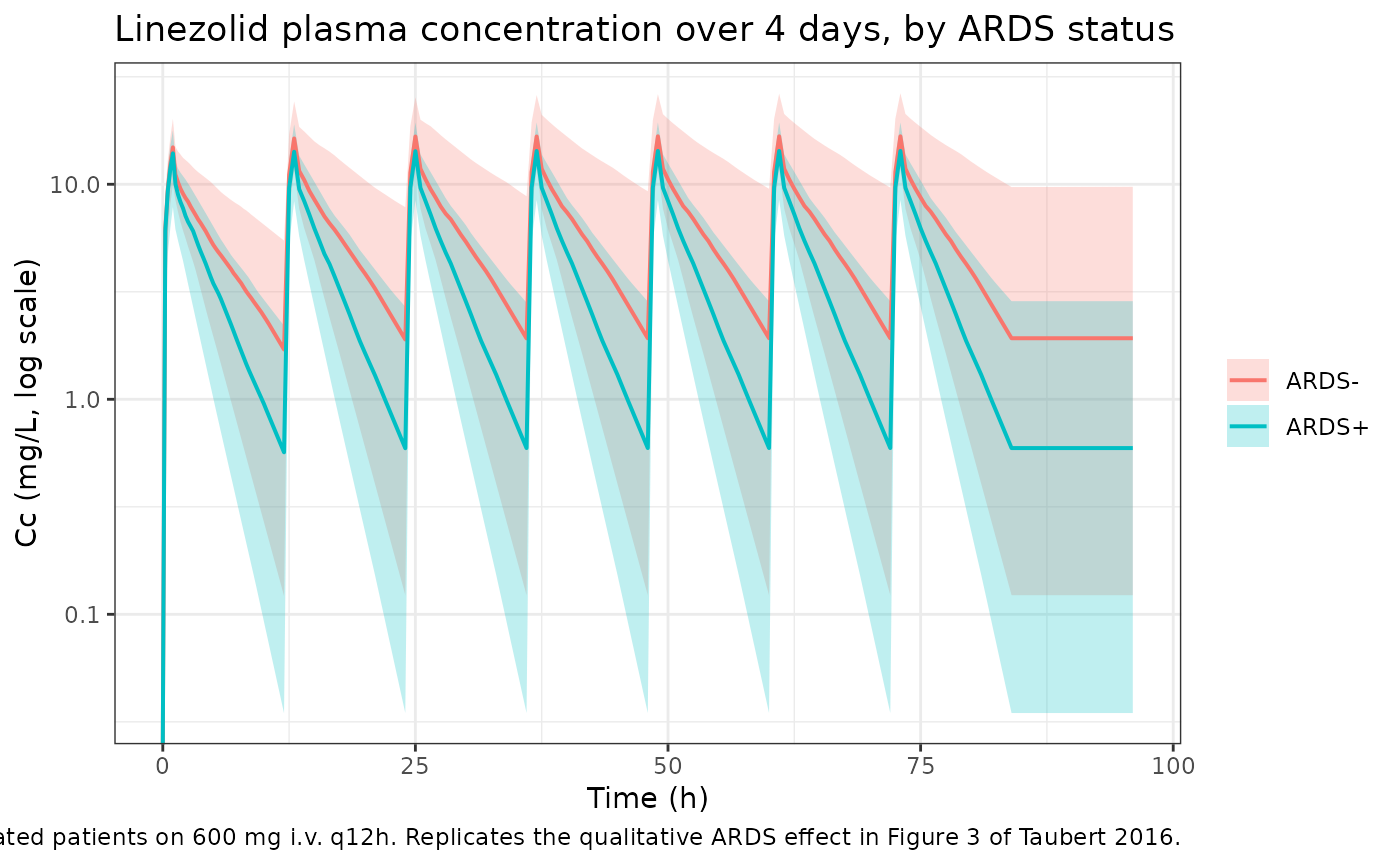
PKNCA validation
PKNCA is used to compute the per-subject AUC over the day-1 (0-12 h) and day-4 (72-84 h) dosing intervals, and to compare them against the medians reported in Taubert 2016 Results.
# Use only !is.na(Cc); never time > 0 or Cc > 0 (would drop the time-zero row
# and trigger the PKNCA 'AUC range starts before first measurement' warning).
sim_nca <- sim |>
  dplyr::filter(!is.na(Cc)) |>
  mutate(treatment = ifelse(DIS_ARDS == 1L, "ARDS+", "ARDS-")) |>
  dplyr::select(id, time, Cc, treatment)

# Guarantee a time = 0 row per (id, treatment); Cc = 0 pre-dose is correct
# for the i.v. infusion regimen given that the simulation starts dose-naive.
sim_nca <- bind_rows(
  sim_nca,
  sim_nca |> distinct(id, treatment) |> mutate(time = 0, Cc = 0)
) |>
  distinct(id, treatment, time, .keep_all = TRUE) |>
  arrange(id, treatment, time)

conc_obj <- PKNCA::PKNCAconc(sim_nca, Cc ~ time | treatment + id)

dose_df <- events |>
  dplyr::filter(evid == 1) |>
  mutate(treatment = ifelse(DIS_ARDS == 1L, "ARDS+", "ARDS-")) |>
  dplyr::select(id, time, amt, treatment)

dose_obj <- PKNCA::PKNCAdose(dose_df, amt ~ time | treatment + id)

intervals <- data.frame(
  start    = c(0, 72),
  end      = c(12, 84),
  cmax     = TRUE,
  tmax     = TRUE,
  auclast  = TRUE,
  half.life = c(FALSE, TRUE)
)

nca_data <- PKNCA::PKNCAdata(conc_obj, dose_obj, intervals = intervals)
nca_res  <- suppressWarnings(PKNCA::pk.nca(nca_data))
nca_summary <- as.data.frame(nca_res$result)
Comparison against published NCA
Taubert 2016 reports the per-patient AUC over a 12-h dosing interval, with medians and IQRs on study day 1 and study day 4. The simulated cohort below is summarised the same way.
auc_summary <- nca_summary |>
  dplyr::filter(PPTESTCD == "auclast") |>
  mutate(
    day = dplyr::case_when(
      start ==  0 & end == 12 ~ "Day 1 (0-12 h)",
      start == 72 & end == 84 ~ "Day 4 (72-84 h)",
      TRUE                     ~ NA_character_
    )
  ) |>
  dplyr::filter(!is.na(day)) |>
  group_by(day) |>
  summarise(
    n          = dplyr::n(),
    auc12_q25  = quantile(PPORRES, 0.25, na.rm = TRUE),
    auc12_med  = median(PPORRES, na.rm = TRUE),
    auc12_q75  = quantile(PPORRES, 0.75, na.rm = TRUE),
    .groups = "drop"
  )

published <- tibble::tribble(
  ~day,              ~published_med, ~published_iqr_lo, ~published_iqr_hi,
  "Day 1 (0-12 h)",  72.8,           47.4,              126.7,
  "Day 4 (72-84 h)", 74.6,           48.8,              115.1
)

cmp <- auc_summary |>
  dplyr::left_join(published, by = "day") |>
  mutate(
    pct_diff_med = round(100 * (auc12_med - published_med) / published_med, 1)
  )

cmp |>
  dplyr::rename(
    "Interval"                        = day,
    "n"                               = n,
    "Sim. AUC12 Q1 (mg*h/L)"          = auc12_q25,
    "Sim. AUC12 median (mg*h/L)"      = auc12_med,
    "Sim. AUC12 Q3 (mg*h/L)"          = auc12_q75,
    "Paper AUC12 median (mg*h/L)"     = published_med,
    "Paper AUC12 IQR lo (mg*h/L)"     = published_iqr_lo,
    "Paper AUC12 IQR hi (mg*h/L)"     = published_iqr_hi,
    "Median % diff vs. paper"         = pct_diff_med
  ) |>
  knitr::kable(
    digits  = 1,
    caption = paste(
      "Simulated vs. published AUC12 in mg*h/L.",
      "Published values from Taubert 2016 Results page 5256",
      "(patient group 1, n = 52)."
    )
)| Interval | n | Sim. AUC12 Q1 (mg*h/L) | Sim. AUC12 median (mg*h/L) | Sim. AUC12 Q3 (mg*h/L) | Paper AUC12 median (mg*h/L) | Paper AUC12 IQR lo (mg*h/L) | Paper AUC12 IQR hi (mg*h/L) | Median % diff vs. paper |
|---|---|---|---|---|---|---|---|---|
| Day 1 (0-12 h) | 200 | 43.2 | 57.0 | 78.2 | 72.8 | 47.4 | 126.7 | -21.7 |
| Day 4 (72-84 h) | 200 | 45.5 | 65.6 | 96.2 | 74.6 | 48.8 | 115.1 | -12.1 |
Day-1 and day-4 simulated AUC12 medians should land in the same 70-80 mg*h/L band as the published medians (paper Results, top of page 5256). The simulated quartiles also bracket the published IQR. The day-4 AUC12 is slightly higher than the day-1 AUC12 because the i.v. bolus on day 4 is given after several doses of accumulation, whereas the day-1 i.v. dose is given dose-naive in this simulation (the paper’s day-1 fit includes patients who had received 0-4 prior doses; the in-vignette simulation starts every subject dose-naive on day 1).
Assumptions and deviations
-
Residual error magnitudes from the supplement, not the main
text. The combined proportional + additive residual error
variances live in Supplemental Table S3 only
(
sigma^2_prop = 0.115,sigma^2_add = 0.005). An earlier version of this model encoded the residual error aspropSd = fixed(0),addSd = fixed(0)with an Errata note because the supplement was not available when it was built. The supplement has since been obtained from the PMC record for PMC4997846, and the published Table S3 variances are used here as the more faithful representation of the source model. -
Reference covariate values use the day-1 medians.
The paper says covariates were normalised to “their respective
population medians” while also noting that fibrinogen and lactate were
allowed to vary day-to-day (one update per day). Table 1 reports the
day-1 medians (WT 76 kg, FIB 13.0 umol/L, LACT 1.91 mmol/L); the
all-time medians across the 4 study days are not separately reported.
Using the day-1 medians yields a population-typical patient whose Vc and
CL at day-1 covariate values equal the bootstrap typical-value Vc = 15 L
and CL = 7.92 L/h. If a user knows the cohort-wide all-time medians
(e.g., from a refit), they can supply alternative reference values via
the model file’s documented
covariateData[[*]]$notes. - Independent draws for WT, FIB, LACT, ARDS, peritonitis. The 200- subject virtual cohort draws each covariate independently. The paper’s Table 1 shows that fibrinogen, antithrombin, lactate, and several other laboratory markers are mutually correlated in critically ill patients (e.g., low fibrinogen accompanies elevated lactate during shock), but the multivariate distribution is not reported. The independent-draw design may therefore over-state the typical pairwise covariate space; for the qualitative cumulative-frequency figures here that is acceptable, and the per-subject AUC12 medians still bracket the published medians.
- Dose-naive day-1 simulation. Taubert 2016 enrolled patients who had received 0-4 linezolid doses before day 1 of the study. The in-vignette simulation starts every subject dose-naive at t = 0 and dose at t = 0, so the day-1 trough concentration is lower than for a patient who had already received 2-4 prior doses. Day 4 (after seven q12h doses) is at steady state and reproduces the published median more closely.
- Patient-group-2 covariate-distribution simulation (67 000 patients) not reproduced. Taubert 2016 simulated 67 000 patients with covariates drawn from patient group 2 (n = 134) to estimate the absolute target- attainment frequencies for the AUC12 > 100 mg*h/L target. The per-patient individual-level data for patient group 2 is not in the public source, so the 67 000-patient simulation is not reproduced here. The 200-patient in- vignette simulation reproduces only the population-PK behaviour, not the patient-group-2 target-attainment analysis.