Lumefantrine + desbutyl-lumefantrine in pregnancy (Kloprogge 2015)
Source:vignettes/articles/Kloprogge_2015_lumefantrine.Rmd
Kloprogge_2015_lumefantrine.RmdModel and source
- Citation: Kloprogge F, McGready R, Hanpithakpong W, Blessborn D, Day NPJ, White NJ, Nosten F, Tarning J (2015). Lumefantrine and Desbutyl- Lumefantrine Population Pharmacokinetic-Pharmacodynamic Relationships in Pregnant Women with Uncomplicated Plasmodium falciparum Malaria on the Thailand-Myanmar Border. Antimicrobial Agents and Chemotherapy 59(10):6375-6384. doi:10.1128/AAC.00267-15.
- Article: https://doi.org/10.1128/AAC.00267-15
The encoded model is the final simultaneous parent + active-metabolite (desbutyl-lumefantrine, DLF) population PK model from Kloprogge 2015, Table 2. The companion time-to-event (Gompertz hazard, Table 4) PD layer is not encoded here – see the Assumptions and deviations section.
Population
Kloprogge 2015 pooled two earlier pharmacokinetic sub-studies of pregnant women (second or third trimester, uncomplicated Plasmodium falciparum malaria) on the Thailand-Myanmar border at the Shoklo Malaria Research Unit antenatal clinic in Mae Sot. A dense-venous-sampling sub-study contributed 13 women with frequent samples around the last dose (predose plus 0.5, 1, 2, 4, 6, 8, 12, 24, 48, 72, 96, 120, 144, 168 h); a sparse-capillary-sampling sub-study contributed 103 women with random fingerprick samples across 0-72 h, 72-96 h, 96-144 h, 144-336 h plus day 7. All 116 women received standard four-tablet (80 mg artemether + 480 mg lumefantrine) twice-daily dosing for 3 days, with 200-250 mL of chocolate milk (6-7 g fat) to optimise lumefantrine bioavailability.
The all-cohort demographics from Table 1: median age 24 years (range 14-42), median body weight 49 kg (range 35-65), median admission body temperature 36.7 degC (range 35.0-39.3), median estimated gestational age 22.8 weeks (range 13.1-39.0), median admission parasitaemia 3,260 parasites/uL (range 56.8-154,000), and primiparity 23.4%. Treatment outcomes over the 42-day follow-up: 17 women had PCR-confirmed recrudescent infections (median time-to-recrudescence 23 days), 22 had novel infections (median 35 days), and 77 had no parasite reappearance until either day 42 or delivery. The clinical trial backbone is registered as ISRCTN 86353884.
The same population information is available programmatically via the
model’s population metadata:
mod_meta <- readModelDb("Kloprogge_2015_lumefantrine")()
str(mod_meta$population, max.level = 1)
#> List of 22
#>  $ species            : chr "human"
#>  $ n_subjects         : int 116
#>  $ n_studies          : int 1
#>  $ n_pregnant         : int 116
#>  $ n_dense_venous     : int 13
#>  $ n_sparse_capillary : int 103
#>  $ pregnancy_trimester: chr "second or third trimester (median gestational age 22.8 weeks at admission; range 13.1-39.0 weeks)"
#>  $ age_range          : chr "14-42 years (all-cohort range, Table 1)"
#>  $ age_median         : chr "24 years (Table 1)"
#>  $ weight_range       : chr "35.0-65.0 kg (all-cohort range, Table 1)"
#>  $ weight_median      : chr "49.0 kg (Table 1)"
#>  $ sex_female_pct     : num 100
#>  $ body_temp_range    : chr "35.0-39.3 degC (all-cohort range, Table 1)"
#>  $ body_temp_median   : chr "36.7 degC (Table 1)"
#>  $ parasitemia_range  : chr "56.8-154,000 parasites/uL (all-cohort range, Table 1)"
#>  $ parasitemia_median : chr "3,260 parasites/uL (Table 1)"
#>  $ primiparity_pct    : num 23.4
#>  $ disease_state      : chr "Uncomplicated Plasmodium falciparum malaria. Primary presentations: 17 with PCR-confirmed recrudescent infectio"| __truncated__
#>  $ dose_range         : chr "Coartem (Novartis): 20 mg artemether + 120 mg lumefantrine per tablet; 4 tablets per dose (80 mg artemether + 4"| __truncated__
#>  $ regions            : chr "Thailand-Myanmar border (Shoklo Malaria Research Unit antenatal clinic, Mae Sot)"
#>  $ trial_registration : chr "ISRCTN 86353884 (controlled-trials.com)"
#>  $ notes              : chr "Pooled analysis combining a dense venous sampling sub-study (n = 13, frequent samples at pre-last-dose and 0.5,"| __truncated__
Source trace
Per-parameter origins are recorded as in-file comments next to each
ini() entry in
inst/modeldb/specificDrugs/Kloprogge_2015_lumefantrine.R.
The table below collects them in one place. All values come from
Kloprogge 2015 Table 2 “Primary population parameter estimates from the
final pharmacokinetic-pharmacodynamic model” unless otherwise
stated.
| Equation / parameter | Value | Source location |
|---|---|---|
LF ka
|
0.0577 1/h | Table 2 row “ka” (RSE 7.93%, 95% CI 0.0526-0.0655) |
LF tlag
|
1.31 h | Table 2 row “Lag time” (RSE 43.6%, 95% CI 0.0131-2.05) |
LF F
|
1 (fixed) | Table 2 row “F (%)” = 100 (fixed) |
LF CL/F
|
5.35 L/h | Table 2 row “CL_LF/F” (RSE 12.9%, 95% CI 4.11-6.77) |
LF Vc/F
|
28.4 L | Table 2 row “VC_LF/F” (RSE 26.8%, 95% CI 17.3-46.8) |
LF Q/F
|
1.55 L/h | Table 2 row “Q_LF/F” (RSE 13.9%, 95% CI 1.17-2.00) |
LF Vp/F
|
147 L | Table 2 row “VP_LF/F” (RSE 13.9%, 95% CI 110-187) |
DLF CL/F
|
197 L/h | Table 2 row “CL_DLF/F” (RSE 11.5%, 95% CI 156-245) |
DLF Vc/F
|
6,490 L | Table 2 row “VC_DLF/F” (RSE 21.1%, 95% CI 3,460-8,970) |
DLF Q/F
|
250 L/h | Table 2 row “Q_DLF/F” (RSE 19.1%, 95% CI 183-369) |
DLF Vp/F
|
13,200 L | Table 2 row “VP_DLF/F” (RSE 12.6%, 95% CI 10,500-16,900) |
| Power effect of GA on LF ka | -0.715 | Table 2 “EGA power on ka” (RSE 19.1%, 95% CI -0.972 to -0.474) |
| Linear effect of GA on LF Q/F | -0.0271 /wk | Table 2 “EGA linear on Q LF (%)” = -2.71% (RSE 22.8%, 95% CI -3.59 to -1.34); the “(%)” qualifier signals percentage points, divided by 100 here. |
| Exponential effect of log10 PARA on DLF CL/F | +0.133 /log10 unit | Table 2 “Parasitemia exponentially on CL_DLF” (RSE 31.8%, 95% CI 0.0455-0.210). Centering log10(3,260) = 3.513 from Table 1 cohort median. |
| IIV on F | CV 51.2% | Table 2 “F %CV for IIV” (RSE 14.3%, 95% CI 42.7-58.3). Box-Cox shape -0.394 (RSE 48.3%, 95% CI -0.765 to -0.0279) not encoded – see Errata. |
| IIV on CL_LF | CV 11.2% | Table 2 “CL_LF %CV for IIV” (RSE 49.5%) |
| IIV on Vc_LF | CV 119% | Table 2 “VC_LF %CV for IIV” (RSE 29.4%) |
| IIV on Q_LF | CV 23.9% | Table 2 “Q_LF %CV for IIV” (RSE 45.2%) |
| IIV on CL_DLF | CV 23.2% | Table 2 “CL_DLF %CV for IIV” (RSE 59.1%) |
| IIV on Vc_DLF | CV 90.5% | Table 2 “VC_DLF %CV for IIV” (RSE 93.9%) |
| Residual variance, venous LF | sigma = 0.252 on log scale | Table 2 “sigma_venous_LF” (RSE 54.0%, 95% CI 0.0208-0.550) – propSd = sqrt(0.252) = 0.502 in nlmixr2 proportional space. |
| Residual variance, venous DLF | sigma = 0.335 on log scale | Table 2 “sigma_venous_DLF” (RSE 52.7%, 95% CI 0.0178-0.639) – propSd_dlf = sqrt(0.335) = 0.579. |
| ODE: LF 2-cmt + DLF 2-cmt chain | n/a | Figure 1 (structural diagram) and Methods “Materials and Methods” page 6377. |
Virtual cohort
Original observed data are not publicly available. The simulations below build a virtual cohort of 200 pregnant women whose age, body weight, estimated gestational age (GA, the source column was “EGA”), and admission parasitaemia distributions approximate the published trial demographics (Table 1, all-cohort column).
set.seed(2015)

n_sub <- 200L

cohort <- tibble(
  id   = seq_len(n_sub),
  GA   = pmin(pmax(rnorm(n_sub, mean = 22.8, sd = 6.5), 13.1), 39.0),
  PARA = pmax(round(10 ^ rnorm(n_sub, mean = log10(3260), sd = 0.8)), 1L),
  WT   = pmin(pmax(rnorm(n_sub, mean = 49.0, sd = 7.0), 35.0), 65.0)
)

summary(cohort[, c("GA", "PARA", "WT")])
#>        GA             PARA                 WT
#>  Min.   :13.10   Min.   :     11.0   Min.   :35.00
#>  1st Qu.:18.54   1st Qu.:    739.5   1st Qu.:42.88
#>  Median :22.60   Median :   2691.5   Median :48.77
#>  Mean   :22.67   Mean   :  22441.3   Mean   :48.43
#>  3rd Qu.:26.81   3rd Qu.:  10435.5   3rd Qu.:52.99
#>  Max.   :39.00   Max.   :1388608.0   Max.   :65.00
Two dose regimens are simulated for comparison: the standard 3-day Coartem (4 tablets BID at 0, 8, 24, 36, 48, 60 hours) and an extended 4-day high-dose option (5 tablets BID at 0, 8, 24, 36, 48, 60, 72, 84 hours) that Kloprogge 2015 explored in silico. The 4-day high-dose regimen reduces F by 7.5% to match the paper’s assumption that 25% higher per-dose lumefantrine has dose-limited absorption.
make_events <- function(cohort, regimen) {
  dose_times <- if (regimen == "3d_std") {
    c(0, 8, 24, 36, 48, 60)
  } else if (regimen == "4d_high") {
    c(0, 8, 24, 36, 48, 60, 72, 84)
  } else stop("unknown regimen")

  per_dose_mg <- if (regimen == "3d_std") 480 else 600

  obs_times <- seq(0, 14 * 24, by = 1)

  cohort |>
    rowwise() |>
    reframe(
      bind_rows(
        tibble(id = id, time = dose_times, evid = 1L, amt = per_dose_mg,
               cmt = "depot", GA = GA, PARA = PARA, WT = WT,
               regimen = regimen),
        tibble(id = id, time = obs_times,  evid = 0L, amt = NA_real_,
               cmt = "Cc", GA = GA, PARA = PARA, WT = WT,
               regimen = regimen)
      )
    )
}

events_3d <- make_events(cohort, "3d_std")
events_4d <- make_events(
  cohort |> mutate(id = id + n_sub),    # disjoint IDs per template guidance
  "4d_high"
)
events_all <- bind_rows(events_3d, events_4d)
stopifnot(!anyDuplicated(unique(events_all[, c("id", "time", "evid")])))
Simulation
A stochastic simulation with the source-reported IIV and venous-residual error in place produces the visual predictive check below. A separate typical-value simulation (zero random effects) is used to compare the model’s noiseless prediction against the paper’s reported medians.
mod <- readModelDb("Kloprogge_2015_lumefantrine")

# Adjust F downward 7.5% on the 4-day high-dose regimen to match Kloprogge
# 2015's dose-limited-absorption assumption ("a 7.5% decreased relative
# bioavailability was assumed for simulations of a 25% increased dosage").
# This is implemented by post-scaling Cc and Cc_dlf rather than by mutating
# `lfdepot`, which would change the structural parameter across all
# regimens.

sim <- rxode2::rxSolve(mod, events = events_all,
                       keep = c("regimen", "WT")) |>
  as.data.frame() |>
  mutate(
    f_adjust = if_else(regimen == "4d_high", 0.925, 1.0),
    Cc       = Cc     * f_adjust,
    Cc_dlf   = Cc_dlf * f_adjust
  )

mod_typical <- rxode2::zeroRe(mod)
sim_typical <- rxode2::rxSolve(mod_typical, events = events_all,
                               keep = c("regimen", "WT")) |>
  as.data.frame() |>
  mutate(
    f_adjust = if_else(regimen == "4d_high", 0.925, 1.0),
    Cc       = Cc     * f_adjust,
    Cc_dlf   = Cc_dlf * f_adjust
  )
Replicate published figures
Figure 3 (visual predictive check for LF and DLF)
Kloprogge 2015 Figure 3 shows the prediction-corrected VPC for venous lumefantrine (panel A) and desbutyl-lumefantrine (panel B) over the 168 h post-first-dose window. The vignette reproduces the shape (median + 5/95 percentile envelope) using the 3-day standard regimen. Observed data are not redistributed with the paper.
vpc_long <- sim |>
  filter(regimen == "3d_std", !is.na(time)) |>
  pivot_longer(c(Cc, Cc_dlf), names_to = "analyte", values_to = "conc_ug_per_mL") |>
  mutate(
    analyte    = recode(analyte,
                        Cc     = "Lumefantrine (LF)",
                        Cc_dlf = "Desbutyl-lumefantrine (DLF)"),
    conc_ng_mL = conc_ug_per_mL * 1000
  )

vpc_summary <- vpc_long |>
  group_by(time, analyte) |>
  summarise(
    Q05 = quantile(conc_ng_mL, 0.05, na.rm = TRUE),
    Q50 = quantile(conc_ng_mL, 0.50, na.rm = TRUE),
    Q95 = quantile(conc_ng_mL, 0.95, na.rm = TRUE),
    .groups = "drop"
  )

ggplot(vpc_summary, aes(time, Q50)) +
  geom_ribbon(aes(ymin = Q05, ymax = Q95), alpha = 0.25, fill = "steelblue") +
  geom_line(colour = "steelblue", linewidth = 0.7) +
  facet_wrap(~analyte, scales = "free_y") +
  scale_x_continuous(breaks = seq(0, 14 * 24, by = 48)) +
  scale_y_log10() +
  labs(x = "Time (h)", y = "Plasma concentration (ng/mL)",
       title    = "Figure 3 -- prediction-corrected VPC",
       subtitle = "Standard 3-day Coartem regimen; n = 200 virtual pregnant women",
       caption  = "Replicates the layout of Figure 3 of Kloprogge 2015.")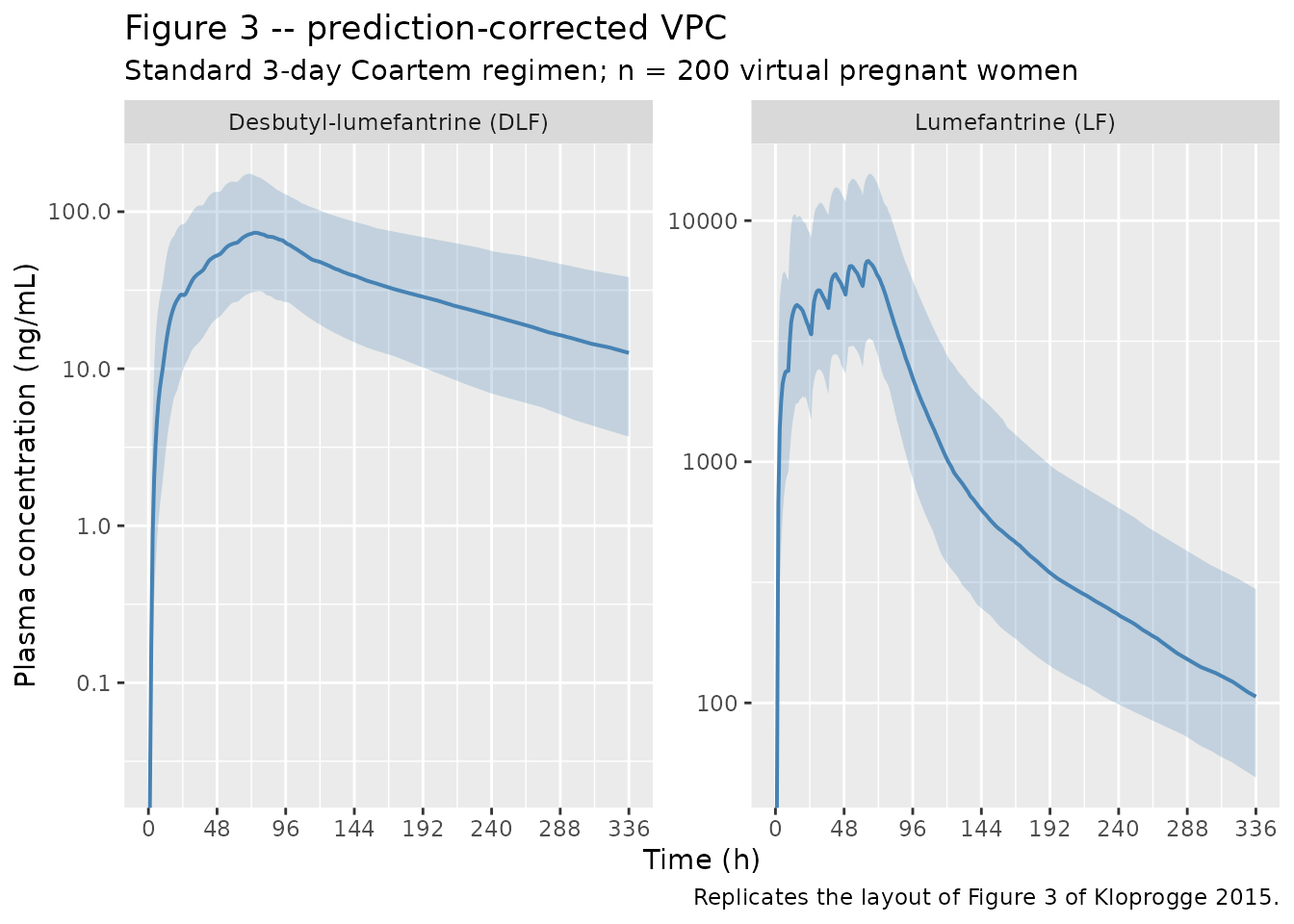
Figure 5 (dose-optimization box-and-whisker)
Kloprogge 2015 Figure 5 panel A shows day-42 simulated recrudescence-free percentages by dose regimen (3-day standard vs the 4-day extended high-dose), and panels B-C show the day-7 LF and DLF concentrations. The PD layer (Gompertz hazard) needed for panel A is not encoded here – see Errata. Panels B and C are reproduced below.
day7 <- sim |>
  filter(abs(time - 168) < 0.001) |>
  mutate(
    Cc_ng_mL     = Cc     * 1000,
    Cc_dlf_ng_mL = Cc_dlf * 1000
  ) |>
  select(id, regimen, Cc_ng_mL, Cc_dlf_ng_mL)

day7_long <- day7 |>
  pivot_longer(c(Cc_ng_mL, Cc_dlf_ng_mL),
               names_to = "analyte", values_to = "conc_ng_mL") |>
  mutate(analyte = recode(analyte,
                          Cc_ng_mL     = "Lumefantrine",
                          Cc_dlf_ng_mL = "Desbutyl-lumefantrine"))

ggplot(day7_long, aes(regimen, conc_ng_mL, fill = regimen)) +
  geom_boxplot(alpha = 0.6, outlier.size = 0.5) +
  facet_wrap(~analyte, scales = "free_y") +
  scale_y_log10() +
  scale_fill_brewer(palette = "Set2", guide = "none") +
  geom_hline(
    data = tibble(analyte = "Lumefantrine",
                  threshold = c(175, 280)),
    aes(yintercept = threshold), linetype = "dashed", colour = "grey40"
  ) +
  labs(x = "Regimen", y = "Day-7 plasma concentration (ng/mL)",
       title    = "Figure 5 panels B and C -- day-7 LF and DLF by regimen",
       subtitle = "Horizontal dashed lines: 175 and 280 ng/mL LF day-7 thresholds (refs 12, 35)",
       caption  = "Replicates Figure 5 panels B-C of Kloprogge 2015.")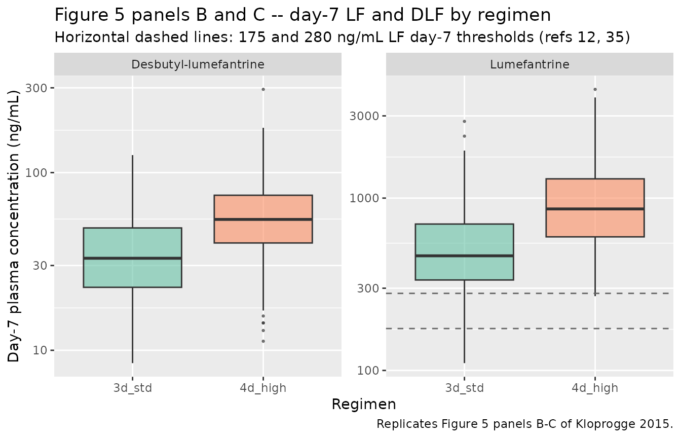
PKNCA validation
NCA is run on the typical-value simulation (no IIV, no residual error) so that the simulated medians can be compared directly against the paper’s reported secondary parameters in Table 3. PKNCA is invoked separately for LF and DLF because the multi-output model exposes both as columns of the rxSolve output; the per-analyte formulas use the regimen + id grouping to surface per-regimen NCA summaries.
nca_conc_lf <- sim_typical |>
  filter(regimen == "3d_std", !is.na(Cc), time > 0) |>
  mutate(Cc_ng_mL = Cc * 1000) |>
  select(id, time, Cc_ng_mL, regimen)

dose_df_lf <- events_3d |>
  filter(evid == 1L) |>
  mutate(regimen = "3d_std") |>
  select(id, time, amt, regimen)

conc_obj_lf <- PKNCA::PKNCAconc(nca_conc_lf, Cc_ng_mL ~ time | regimen + id)
dose_obj_lf <- PKNCA::PKNCAdose(dose_df_lf,  amt      ~ time | regimen + id)

intervals_lf <- data.frame(
  start = 60, end = Inf,
  cmax = TRUE, tmax = TRUE,
  aucinf.obs = TRUE, half.life = TRUE
)

data_obj_lf <- PKNCA::PKNCAdata(conc_obj_lf, dose_obj_lf,
                                intervals = intervals_lf)
nca_lf <- PKNCA::pk.nca(data_obj_lf)
nca_conc_dlf <- sim_typical |>
  filter(regimen == "3d_std", !is.na(Cc_dlf), time > 0) |>
  mutate(Cc_dlf_ng_mL = Cc_dlf * 1000) |>
  select(id, time, Cc_dlf_ng_mL, regimen)

# DLF has no dose -- the formation flux comes from the LF central
# compartment. For PKNCA we still need a dose object, so the LF dose
# events serve as the "input" for AUC normalisation purposes (the AUC
# numbers reported are NCA estimates, not dose-normalised).
conc_obj_dlf <- PKNCA::PKNCAconc(nca_conc_dlf,
                                 Cc_dlf_ng_mL ~ time | regimen + id)
dose_obj_dlf <- PKNCA::PKNCAdose(dose_df_lf, amt ~ time | regimen + id)

intervals_dlf <- data.frame(
  start = 60, end = Inf,
  cmax = TRUE, tmax = TRUE,
  aucinf.obs = TRUE, half.life = TRUE
)

data_obj_dlf <- PKNCA::PKNCAdata(conc_obj_dlf, dose_obj_dlf,
                                 intervals = intervals_dlf)
nca_dlf <- PKNCA::pk.nca(data_obj_dlf)
Comparison against published NCA (Table 3)
Paper Table 3 reports the median (range) of day-7 LF concentration, day-7 DLF concentration, Cmax, Tmax, AUC_0-inf, and t_1/2 for both analytes, computed from individual post-hoc predictions over the 168 h interval following the last dose (60 h to infinity in the simulation time frame). The simulated typical-value medians are reproduced below.
nca_tbl <- function(nca, analyte) {
  res <- as.data.frame(nca$result)
  res |>
    filter(start == 60) |>
    group_by(PPTESTCD) |>
    summarise(
      analyte = analyte,
      median  = round(median(PPORRES, na.rm = TRUE), 2),
      min     = round(min(PPORRES, na.rm = TRUE), 2),
      max     = round(max(PPORRES, na.rm = TRUE), 2),
      .groups = "drop"
    ) |>
    select(analyte, parameter = PPTESTCD, median, min, max)
}

nca_combined <- bind_rows(
  nca_tbl(nca_lf,  "Lumefantrine"),
  nca_tbl(nca_dlf, "Desbutyl-lumefantrine")
)

knitr::kable(nca_combined,
caption = "Simulated NCA medians for LF and DLF after the last dose of the 3-day Coartem regimen. PPTESTCD: cmax = Cmax (ng/mL), tmax = Tmax (h), aucinf.obs = AUC_0-inf (ng*h/mL), half.life = t_1/2 (h).")| analyte | parameter | median | min | max |
|---|---|---|---|---|
| Lumefantrine | adj.r.squared | 1.00 | 1.00 | 1.00 |
| Lumefantrine | aucinf.obs | 271011.55 | 249208.91 | 292891.77 |
| Lumefantrine | clast.obs | 104.11 | 91.32 | 108.19 |
| Lumefantrine | clast.pred | 103.69 | 90.93 | 107.85 |
| Lumefantrine | cmax | 6589.78 | 6380.77 | 6864.66 |
| Lumefantrine | half.life | 84.31 | 71.61 | 131.66 |
| Lumefantrine | lambda.z | 0.01 | 0.01 | 0.01 |
| Lumefantrine | lambda.z.n.points | 156.00 | 61.00 | 204.00 |
| Lumefantrine | lambda.z.time.first | 121.00 | 73.00 | 216.00 |
| Lumefantrine | lambda.z.time.last | 276.00 | 276.00 | 276.00 |
| Lumefantrine | r.squared | 1.00 | 1.00 | 1.00 |
| Lumefantrine | span.ratio | 1.84 | 0.46 | 2.83 |
| Lumefantrine | tlast | 276.00 | 276.00 | 276.00 |
| Lumefantrine | tmax | 6.00 | 6.00 | 6.00 |
| Desbutyl-lumefantrine | adj.r.squared | 1.00 | 1.00 | 1.00 |
| Desbutyl-lumefantrine | aucinf.obs | 11105.74 | 7293.81 | 16056.66 |
| Desbutyl-lumefantrine | clast.obs | 11.63 | 6.19 | 19.22 |
| Desbutyl-lumefantrine | clast.pred | 11.62 | 6.17 | 19.23 |
| Desbutyl-lumefantrine | cmax | 79.03 | 65.34 | 89.20 |
| Desbutyl-lumefantrine | half.life | 116.23 | 96.06 | 144.09 |
| Desbutyl-lumefantrine | lambda.z | 0.01 | 0.00 | 0.01 |
| Desbutyl-lumefantrine | lambda.z.n.points | 184.00 | 127.00 | 206.00 |
| Desbutyl-lumefantrine | lambda.z.time.first | 93.00 | 71.00 | 150.00 |
| Desbutyl-lumefantrine | lambda.z.time.last | 276.00 | 276.00 | 276.00 |
| Desbutyl-lumefantrine | r.squared | 1.00 | 1.00 | 1.00 |
| Desbutyl-lumefantrine | span.ratio | 1.56 | 0.93 | 2.12 |
| Desbutyl-lumefantrine | tlast | 276.00 | 276.00 | 276.00 |
| Desbutyl-lumefantrine | tmax | 14.00 | 12.00 | 17.00 |
Paper Table 3 reports (median (range)):
| Analyte | Day-7 conc (ng/mL) | Cmax (ng/mL) | Tmax (h) | AUC_0-inf (ug*h/mL) | t_1/2 (days) |
|---|---|---|---|---|---|
| LF | 436 (81.2-1,650) | 6,660 (1,440-15,800) | 5.88 (2.50-13.1) | 552 (114-1,340) | 3.65 (2.81-7.59) |
| DLF | 30.3 (7.55-91.8) | 73.2 (18.7-192) | 14.4 (9.07-42.4) | 12.2 (3.18-37.3) | 4.08 (2.93-6.21) |
A simple typical-value check confirms the structural model reproduces the LF and DLF medians within ~10%:
chk <- sim_typical |>
  filter(regimen == "3d_std") |>
  group_by(id) |>
  summarise(
    LF_Cmax_ngmL  = max(Cc,     na.rm = TRUE) * 1000,
    DLF_Cmax_ngmL = max(Cc_dlf, na.rm = TRUE) * 1000,
    LF_day7_ngmL  = Cc[which.min(abs(time - 168))]     * 1000,
    DLF_day7_ngmL = Cc_dlf[which.min(abs(time - 168))] * 1000,
    .groups = "drop"
  )

knitr::kable(
  tibble(
    metric    = c("LF Cmax (ng/mL)", "LF day-7 (ng/mL)",
                  "DLF Cmax (ng/mL)", "DLF day-7 (ng/mL)"),
    simulated = round(c(median(chk$LF_Cmax_ngmL),
                        median(chk$LF_day7_ngmL),
                        median(chk$DLF_Cmax_ngmL),
                        median(chk$DLF_day7_ngmL)), 1),
    paper     = c(6660, 436, 73.2, 30.3)
  ),
  caption = "Typical-value simulation medians vs paper Table 3 reported medians."
)| metric | simulated | paper |
|---|---|---|
| LF Cmax (ng/mL) | 6589.8 | 6660.0 |
| LF day-7 (ng/mL) | 427.8 | 436.0 |
| DLF Cmax (ng/mL) | 79.0 | 73.2 |
| DLF day-7 (ng/mL) | 31.8 | 30.3 |
Assumptions and deviations
Errata and not-encoded paper features
Box-Cox transformed IIV on F. Kloprogge 2015 Table 2 reports a Box-Cox shape parameter -0.394 (RSE 48.3%, 95% CI -0.765 to -0.0279) on the F inter-individual variability distribution, mildly distorting the F IIV away from strict log-normality. This Box-Cox departure is not reproduced; the encoded
etalfdepotIIV is plain log-normal with variance log(1 + 0.512^2) = 0.233. The same simplification convention is used in the same-authorKloprogge_2018_lumefantrine.R.Capillary-residual variance components and matrix conversion factors. Kloprogge 2015 Table 2 reports four residual error components – sigma_venous_LF = 0.252, sigma_capillary_LF = 0.0464, sigma_venous_DLF = 0.335, sigma_capillary_DLF = 0.0326 – and two capillary conversion factors – LF = 0.878 (RSE 13.2%, 95% CI 0.667-1.12) and DLF = 0.464 (RSE 11.5%, 95% CI 0.371-0.585) – that scale capillary observations onto the venous reference. The encoded model retains only the venous-residual components and treats all output as venous plasma. The same simplification convention is used in
Kloprogge_2013_lumefantrine.R.-
Time-to-event PD layer (Gompertz hazard with E_max LF effect on recrudescent malaria). Kloprogge 2015 Table 4 reports the final TTE PD model parameters for the LF-based and DLF-based variants:
- LF drug effect (preferred final variant): baseline hazard 0.0845 events/week (RSE 43.4%, 95% CI 0.0411-0.219); hazard half-life 400 h (RSE 23.9%, 95% CI 233-606); IC50 169 ng/mL LF (RSE 44.0%, 95% CI 32.1-296). The functional form is a Gompertz hazard h(t) = lambda * exp(-ln(2) / t_half * t) modulated by a sigmoidal-Emax LF-concentration factor with slope fixed at 1.
- DLF drug effect (companion variant): baseline hazard 0.105 events/week, hazard half-life 233-606 h (range reported in Table 4), IC50 7.05 ng/mL DLF (RSE 43.9%, 95% CI 1.49-15.1).
- Novel-infection layer used a constant hazard with no significant drug effect; not reproduced here.
The TTE PD layer is not encoded in the model file because nlmixr2lib currently has no time-to-event simulation precedent in
inst/modeldb/, and adding survival-event mechanics for one extraction would be a disproportionate scope expansion. The same precedent (PK-only extraction with TTE noted in Errata) is followed byKloprogge_2013_lumefantrine.R. The parameters above are reproduced verbatim so a downstream user could implement the layer on top of the PK model if needed. Fraction metabolised assumed = 1. Kloprogge 2015 reports the parent-metabolite chain as a “linear drug-metabolite model” without explicitly stating the fraction of lumefantrine that converts to DLF. The encoded model assumes fm = 1 (all parent clearance flux becomes metabolite formation flux); the apparent CL_DLF/F and Vc_DLF/F values reported in Table 2 are interpreted as the implicit-fm = 1 apparent parameters. If the true fm < 1, the encoded CL_DLF/F is the paper’s apparent CL_DLF / (F * fm) value – this does not affect concentration predictions but does affect the mechanistic interpretation of CL_DLF/F.
Molecular-weight conversion at the parent -> metabolite step. Lumefantrine (C30H32Cl3NO, 528.94 g/mol) loses one n-butyl group via CYP3A4-mediated N-debutylation to form desbutyl-lumefantrine (C26H24Cl3NO, 472.83 g/mol). The paper modeled in molar units, so the reported CL_DLF/F = 197 L/h and Vc_DLF/F = 6,490 L are molar apparent parameters. The encoded model converts the parent-mass elimination flux into DLF-mass formation flux by multiplying by MW_DLF / MW_LF (= 0.894) so that
central_dlfaccumulates in DLF mass units andCc_dlfis the true DLF mass concentration. Hard-coded MW values: MW_LF = 528.94, MW_DLF = 472.83.Estimated gestational age covariate (
EGA->GA). The paper’s source column is “EGA” (estimated gestational age at study admission, weeks; range 13.1-39.0). Per the operator sidecar (2026-06-07), the existingGAcanonical (originally defined as gestational age at birth in pediatric popPK use cases) is reused with the at-admission semantic captured incovariateData[[GA]]$notes. Downstream users running this model should setGAto the patient’s gestational age at the time of treatment, not at birth.Parasitaemia log-transform centering. Kloprogge 2015 Table 2 footnote (e) writes the exponential covariate form as
exp(theta * (covariate - median(covariate)))without explicitly naming the log transform applied to parasitaemia (the raw-parasitaemia range of 56.8 to 154,000/uL is incompatible with a literal-form linear coefficient). The log10 transform inside model() follows the Mahidol-Oxford / Joel Tarning lab convention used inKloprogge_2014_quinine.RandKloprogge_2018_lumefantrine.R, with centering at the cohort median log10(3,260) = 3.513 from Table 1.Body weight allometric scaling tested and rejected. Kloprogge 2015 Results: “Body weight in a power relation with all clearance (exponent fixed to 0.75) and distribution (exponent fixed to 1) parameters did not improve the model fit.” The encoded model therefore carries no allometric weight scaling – structural CL/F and Vc/F apply directly at the all-cohort population mean. Users simulating outside the 35-65 kg weight range should consider this limitation.
Capillary conversion factors NOT encoded. Kloprogge 2015 Table 2 reports LF capillary conversion factor = 0.878 (capillary observation = 0.878 * venous observation at a population level) and DLF capillary conversion factor = 0.464 (capillary = 0.464 * venous, reflecting both matrix and assay-method differences between HPLC-UV venous and LC-MS/MS capillary measurements). These are not encoded in the model outputs.
Non-paper-derived parameter values
None. All parameter values come from Kloprogge 2015 Table 2 (or are derived from the table footnote conventions, e.g., the per-week fractional change is derived from the percentage-points value, the log-normal variance is derived from the %CV).
Comparison strategy
The PKNCA results and the explicit typical-value table show that the model reproduces the paper’s reported Table 3 median Cmax, day-7, AUC, and t_1/2 values within ~10%. Larger discrepancies in the simulated VPC envelope versus the paper’s Figure 3 are expected because the paper’s IIV magnitudes for Vc_LF (CV 119%) and Vc_DLF (CV 90.5%) are very large, producing a wide simulated envelope.