Colistin sulfate (Xie 2022)
Source:vignettes/articles/Xie_2022_colistinSulfate.Rmd
Xie_2022_colistinSulfate.RmdModel and source
- Citation: Xie Y-L, Jin X, Yan S-S, Wu C-F, Xiang B-X, Wang H, Liang W, Yang B-C, Xiao X-F, Li Z-L, Pei Q, Zuo X-C, Peng Y (2022). Population pharmacokinetics of intravenous colistin sulfate and dosage optimization in critically ill patients. Front Pharmacol 13:967412. doi:10.3389/fphar.2022.967412.
- Description: Two-compartment population PK model for intravenous colistin sulfate in critically ill Chinese adults (Xie 2022; n = 20 ICU patients, 98 plasma concentrations collected after at least 72 h of therapy). Linear elimination from the central compartment with a 1-2 h intravenous infusion input. Cockcroft-Gault creatinine clearance enters clearance as a power function centred on 57.5 mL/min (exponent 0.353) and alanine aminotransferase enters the peripheral volume as a power function centred on 37 U/L (exponent 0.635). Inter-individual variability on CL and the central volume only; proportional residual error. Colistin sulfate is administered as the active drug and must not be confused with colistimethate sodium (CMS), the inactive prodrug. Dose unit conversion: 10,000 IU = 0.44 mg, so 1 million units (MU) = 44 mg.
- Article: https://doi.org/10.3389/fphar.2022.967412 (open access)
Values come from the main text (Table 2 and Eqs 1-3) and from the supplementary material (Data Sheet 1: Supplementary Tables S1-S3). No erratum was found for this article (Europe PMC correction links for PMID 36105229, checked 2026-10-09).
Colistin sulfate is the active polymyxin E salt,
given intravenously as such. It is not colistimethate sodium (CMS), the
inactive prodrug modelled in this library by
Plachouras_2009_colistin,
Mohamed_2012_colistin, Jacobs_2016_colistin
and Karaiskos_2015_colistin. Other colistin sulfate models
in the library are Huang_2025_colistinSulfate,
Sun_2025_colistinSulfate,
Ma_2026_colistinSulfate and
Jin_2026_colistinSulfate.
Population
Twenty critically ill adults treated with intravenous colistin sulfate for at least 72 h in the ICU of the Third Xiangya Hospital of Central South University (Changsha, China) between May 2021 and April 2022 (Table 1). Median age was 60.5 years (range 18-92), 8 of 20 were female, and median total body weight was 55 kg (45-65). Cockcroft-Gault creatinine clearance (CrCL) had a median of 48.8 mL/min and spanned 6.5-193.8 mL/min; two patients were on continuous renal replacement therapy. Alanine aminotransferase (ALT) had a median of 37.5 U/L and spanned 7-495 U/L, and 65% had underlying liver disease. Median APACHE II score was 21.5 and median SOFA score 8. Carbapenem-resistant A. baumannii (50%) and K. pneumoniae (30%) were the main isolates, and 80% of patients received concomitant meropenem.
Doses were 1.0-2.0 million IU (MU) per day, most often 1.5 MU/day, split into 2 or 3 infusions of 1-2 h; four patients received a loading dose. The paper’s conversion is 10,000 IU = 0.44 mg, so 1 MU = 44 mg. Ninety-eight plasma concentrations were collected after at least 72 h of therapy (38 troughs, 27 peaks, 33 random samples). The model was fitted in Phoenix NLME 8.3.4 with FOCE-ELS.
The same information is available programmatically via
readModelDb("Xie_2022_colistinSulfate")()$population.
Source trace
| Equation / parameter | Value | Source location |
|---|---|---|
lcl (CL, L/h) |
1.50 | Table 2 tvCL (CV 11.7%); Eq. 3 |
lvc (V, L) |
16.1 | Table 2 tvV (CV 8.70%); Eq. 1 |
lvp (V2, L) |
50.5 | Table 2 tvV2 (CV 22.0%); Eq. 2 |
lq (CL2, L/h) |
1.71 | Table 2 tvCL2 (CV 22.0%); Results text “estimated as
1.71 L/h with no inter-individual variability” |
e_crcl_cl |
0.353 | Table 2 dCLdCrCL (CV 29.8%); Eq. 3 exponent |
e_alt_vp |
0.635 | Table 2 dV2dALT (CV 16.6%); Eq. 2 exponent |
| CrCL centring constant | 57.5 mL/min | Eq. 3 only; not tabulated |
| ALT centring constant | 37 U/L | Eq. 2 only; not tabulated |
etalcl |
0.197 | Table 2 omega2 CL (variance) |
etalvc |
0.0267 | Table 2 omega2 V (variance) |
propSd |
0.228 | Table 2 stdev0; Results “a proportional error
model” |
cl <- exp(lcl + etalcl) * (CRCL / 57.5)^e_crcl_cl |
n/a | Eq. 3 |
vc <- exp(lvc + etalvc) |
n/a | Eq. 1 |
vp <- exp(lvp) * (ALT / 37)^e_alt_vp |
n/a | Eq. 2 |
| two-compartment ODEs, linear elimination | n/a | Results “a two-compartment model with first-order elimination” |
Cc ~ prop(propSd) |
n/a | Results; Table 2 stdev0
|
Table 2’s “CV (%)” column is the precision of each estimate; its legend expands it as “percent confidence of variation”.
Inter-individual variability scale from the paper’s own Table 3
Table 2 labels the IIV rows omega2 and its legend calls
them the “variance of inter-individual variability”, so
etalcl ~ 0.197 is a variance (an SD of 0.444 on the log
scale). The paper’s Table 3 – the probability that the average
steady-state concentration exceeds 2 or 4 mg/L for 12 regimens at four
CrCL values – gives an independent check that does not depend on the
clearance level or on the dose conversion.
For a log-normal CL at fixed CrCL,
qnorm(P(Css,avg > C)) is linear in
log(daily dose / C) with slope 1 / omega.
Differencing two maintenance-only regimens (or the two thresholds) in
the same CrCL column cancels the typical clearance and leaves
omega.
# Xie 2022 Table 3, transcribed verbatim (percent). `ld_mu` is the loading dose
# and `md_mu` the maintenance dose, both in MU; `tau` is the interval in hours.
table3 <- tibble::tibble(
  regimen = c("0.5MU q12h", "1.0MU + 0.5MU q12h", "1.5MU + 0.5MU q12h",
              "0.5MU q8h", "0.75MU q12h", "1.0MU + 0.5MU q8h",
              "1.0MU + 0.75MU q12h", "1.5MU + 0.5MU q8h",
              "1.5MU + 0.75MU q12h", "1.0 MU q12h", "1.5MU + 1.0 MU q12h",
              "1.0MU + 0.75MU q8h"),
  ld_mu = c(0, 1, 1.5, 0, 0, 1, 1, 1.5, 1.5, 0, 1.5, 1),
  md_mu = c(0.5, 0.5, 0.5, 0.5, 0.75, 0.5, 0.75, 0.5, 0.75, 1, 1, 0.75),
  tau = c(12, 12, 12, 8, 12, 8, 12, 8, 12, 12, 12, 8)
) |>
  mutate(daily_mu = md_mu * 24 / tau)

p_gt2 <- rbind(
  c(74, 29, 21, 15), c(85.5, 37.5, 28, 17), c(94, 53, 42, 33),
  c(96.5, 75, 62.5, 49), c(96.5, 73.5, 58, 45), c(98, 77, 69.5, 56.5),
  c(98, 70, 59, 43.5), c(98.5, 82, 68.5, 57), c(97.5, 81, 65.5, 52.5),
  c(99.5, 88.5, 78, 69), c(100, 87, 79.5, 71.5), c(100, 93, 87, 80.5)
)
p_gt4 <- rbind(
  c(4, 0, 0, 0), c(7.5, 0.5, 0, 0), c(28.5, 3, 1.5, 1.5),
  c(46, 7, 2.5, 1), c(41, 7, 2.5, 0.5), c(56, 16.5, 12.5, 7.5),
  c(44.5, 12, 6, 3), c(66.5, 20, 12, 7.5), c(59.5, 14.5, 7.5, 4.5),
  c(76, 33, 23, 13), c(79, 39, 26.5, 16.5), c(87, 55.5, 36.5, 28.5)
)
crcl_grid <- c(10, 50, 80, 120)

table3_long <- bind_rows(
  table3 |> mutate(thr = 2) |> bind_cols(as.data.frame(p_gt2)),
  table3 |> mutate(thr = 4) |> bind_cols(as.data.frame(p_gt4))
) |>
  tidyr::pivot_longer(V1:V4, names_to = "col", values_to = "pct") |>
  mutate(CRCL = crcl_grid[as.integer(sub("V", "", col))]) |>
  select(-col)

stopifnot(nrow(table3_long) == 96)
# Maintenance-only rows: a loading dose changes Table 3 (see below), so only
# rows without one are comparable across daily doses. Cells at 0% or 100%
# carry no information about the spread.
informative <- table3_long |>
  filter(ld_mu == 0, pct > 0.1, pct < 99.9) |>
  mutate(z = qnorm(pct / 100), x = log(daily_mu / thr))

omega_pairs <- informative |>
  group_by(CRCL) |>
  group_modify(function(g, key) {
    p <- utils::combn(nrow(g), 2)
    tibble::tibble(
      same_thr = g$thr[p[2, ]] == g$thr[p[1, ]],
      dx = g$x[p[2, ]] - g$x[p[1, ]],
      dz = g$z[p[2, ]] - g$z[p[1, ]]
    )
  }) |>
  ungroup() |>
  filter(abs(dx) > 0.1) |>
  mutate(omega_hat = dx / dz)

omega_same <- median(omega_pairs$omega_hat[omega_pairs$same_thr])
omega_hat <- median(omega_pairs$omega_hat)

tibble::tibble(
  Quantity = c("pairs at the same threshold (dose ratio only)",
               "all pairs (dose ratio and threshold ratio)",
               "omega if omega2 CL = 0.197 is a variance",
               "omega if 0.197 were an SD"),
  n = c(sum(omega_pairs$same_thr), nrow(omega_pairs), NA, NA),
  omega = c(omega_same, omega_hat, sqrt(0.197), 0.197)
) |>
  knitr::kable(digits = 3, caption = paste(
    "IIV on CL recovered from Xie 2022 Table 3 by the dose-ratio probit",
    "identity (median over pairs). Arithmetic on published numbers, not a",
    "simulation."
))| Quantity | n | omega |
|---|---|---|
| pairs at the same threshold (dose ratio only) | 31 | 0.359 |
| all pairs (dose ratio and threshold ratio) | 79 | 0.347 |
| omega if omega2 CL = 0.197 is a variance | NA | 0.444 |
| omega if 0.197 were an SD | NA | 0.197 |
# Deterministic arithmetic on printed numbers. On the log scale both
# estimates sit nearer the variance reading (0.444) than the SD reading
# (0.197).
stopifnot(
  abs(log(omega_same / sqrt(0.197))) < abs(log(omega_same / 0.197)),
  abs(log(omega_hat / sqrt(0.197))) < abs(log(omega_hat / 0.197))
)
Pairs at the same threshold, which depend only on the dose ratio,
return omega = 0.359, and all pairs together return 0.347.
Both fall between the two readings, nearer the variance reading
(sqrt(0.197) = 0.444) than the SD reading (0.197) on the
log scale. The table therefore does not pin omega as
sharply as the Table 2 header does, but it does not contradict the
header either. The estimate is not exact because the paper’s Css,avg is
not a pure steady-state, log-normal quantity (it changes with the
loading dose; see below).
Virtual cohort and simulation
The cohort follows the paper’s Monte Carlo design: four fixed CrCL values (10, 50, 80 and 120 mL/min), 2-h infusions and doses converted at 1 MU = 44 mg. ALT is held at the 37 U/L reference because the paper’s simulations do not state an ALT value (ALT acts only on V2 and does not change the steady-state average concentration). Two regimens are simulated over the first three days, the paper’s lowest (0.5 MU q12h, no loading dose) and its recommended regimen for CrCL 50 mL/min (1.5 MU loading dose then 0.5 MU q8h). A third set solves 0.5 MU q12h directly at steady state.
# set.seed() seeds R's RNG only. rxode2's simulation RNG is partitioned per
# solver thread, so the drawn cohort can differ between machines; every
# assertion on a cohort-derived quantity below is written to hold for any
# such cohort.
set.seed(20221009)
mg_per_mu <- 44 # 10,000 IU = 0.44 mg (Methods; Table 3 footnote)
n_per_arm <- 200

make_course <- function(label, ld_mu, md_mu, tau, crcl, id_offset) {
  subj <- tibble::tibble(id = id_offset + seq_len(n_per_arm), CRCL = crcl,
                         ALT = 37, regimen = label)
  md_times <- if (ld_mu > 0) seq(tau, 72 - tau, by = tau) else seq(0, 72 - tau, by = tau)
  dose_tbl <- tibble::tibble(time = md_times, amt = md_mu * mg_per_mu)
  if (ld_mu > 0) dose_tbl <- bind_rows(tibble::tibble(time = 0, amt = ld_mu * mg_per_mu), dose_tbl)
  doses <- subj |>
    tidyr::crossing(dose_tbl) |>
    mutate(evid = 1L, rate = amt / 2, cmt = "central")
  obs <- subj |>
    tidyr::crossing(time = seq(0, 72, by = 0.25)) |>
    mutate(evid = 0L, amt = NA_real_, rate = NA_real_, cmt = "central")
  bind_rows(doses, obs) |> arrange(id, time, desc(evid))
}

course_arms <- tidyr::crossing(
  tibble::tibble(label = c("0.5MU q12h", "1.5MU + 0.5MU q8h"),
                 ld_mu = c(0, 1.5), md_mu = c(0.5, 0.5), tau = c(12, 8)),
  CRCL = crcl_grid
) |>
  mutate(id_offset = (row_number() - 1L) * n_per_arm)

events_course <- bind_rows(lapply(seq_len(nrow(course_arms)), function(i) {
  a <- course_arms[i, ]
  make_course(a$label, a$ld_mu, a$md_mu, a$tau, a$CRCL, a$id_offset)
}))

# Steady state: one ss = 1 infusion record per subject, then one interval.
make_ss <- function(crcl, id_offset) {
  subj <- tibble::tibble(id = id_offset + seq_len(n_per_arm), CRCL = crcl,
                         ALT = 37, regimen = "0.5MU q12h (steady state)")
  doses <- subj |>
    mutate(time = 0, amt = 0.5 * mg_per_mu, rate = amt / 2, ii = 12, ss = 1L,
           evid = 1L, cmt = "central")
  obs <- subj |>
    tidyr::crossing(time = seq(0, 12, by = 0.25)) |>
    mutate(evid = 0L, amt = NA_real_, rate = NA_real_, ii = 0, ss = 0L,
           cmt = "central")
  bind_rows(doses, obs) |> arrange(id, time, desc(evid))
}
events_ss <- bind_rows(lapply(seq_along(crcl_grid), function(i) {
  make_ss(crcl_grid[i], 10000L + (i - 1L) * n_per_arm)
}))

stopifnot(
  !anyDuplicated(events_course[events_course$evid == 0, c("id", "time")]),
  length(unique(events_course$id)) == 8 * n_per_arm,
  length(unique(events_ss$id)) == 4 * n_per_arm
)
mod <- readModelDb("Xie_2022_colistinSulfate")

sim_course <- rxode2::rxSolve(
  mod, events = events_course, keep = c("regimen", "CRCL"), maxsteps = 1e6
) |>
  as.data.frame()
#> ℹ parameter labels from comments will be replaced by 'label()'

# A subject with low CL at CrCL 10 mL/min has a terminal half-life of several
# hundred hours, so the steady-state search needs a large step budget and
# tight steady-state tolerances.
sim_ss <- rxode2::rxSolve(
  mod, events = events_ss, keep = c("regimen", "CRCL"), maxsteps = 1e6,
  rtol = 1e-8, atol = 1e-10, ssRtol = 1e-8, ssAtol = 1e-10
) |>
  as.data.frame()

stopifnot(
  !anyNA(sim_course$Cc), !anyNA(sim_ss$Cc),
  all(sim_course$Cc >= -1e-6 * max(sim_course$Cc)),
  all(sim_ss$Cc >= -1e-6 * max(sim_ss$Cc))
)
Typical-value profiles
mod_typ <- rxode2::zeroRe(mod)
#> ℹ parameter labels from comments will be replaced by 'label()'
typ_events <- events_course |>
  filter(id %in% (course_arms$id_offset + 1L))
sim_typ <- rxode2::rxSolve(mod_typ, events = typ_events,
                           keep = c("regimen", "CRCL")) |>
  as.data.frame()
#> ℹ omega/sigma items treated as zero: 'etalcl', 'etalvc'
#> Warning: multi-subject simulation without without 'omega'

ggplot(sim_typ, aes(time, Cc, colour = factor(CRCL))) +
  geom_line() +
  facet_wrap(~regimen) +
  labs(x = "Time (h)", y = "Colistin concentration (mg/L)",
       colour = "CrCL (mL/min)",
       title = "Typical-value profiles over the first three days",
       caption = "2-h infusions, ALT = 37 U/L.")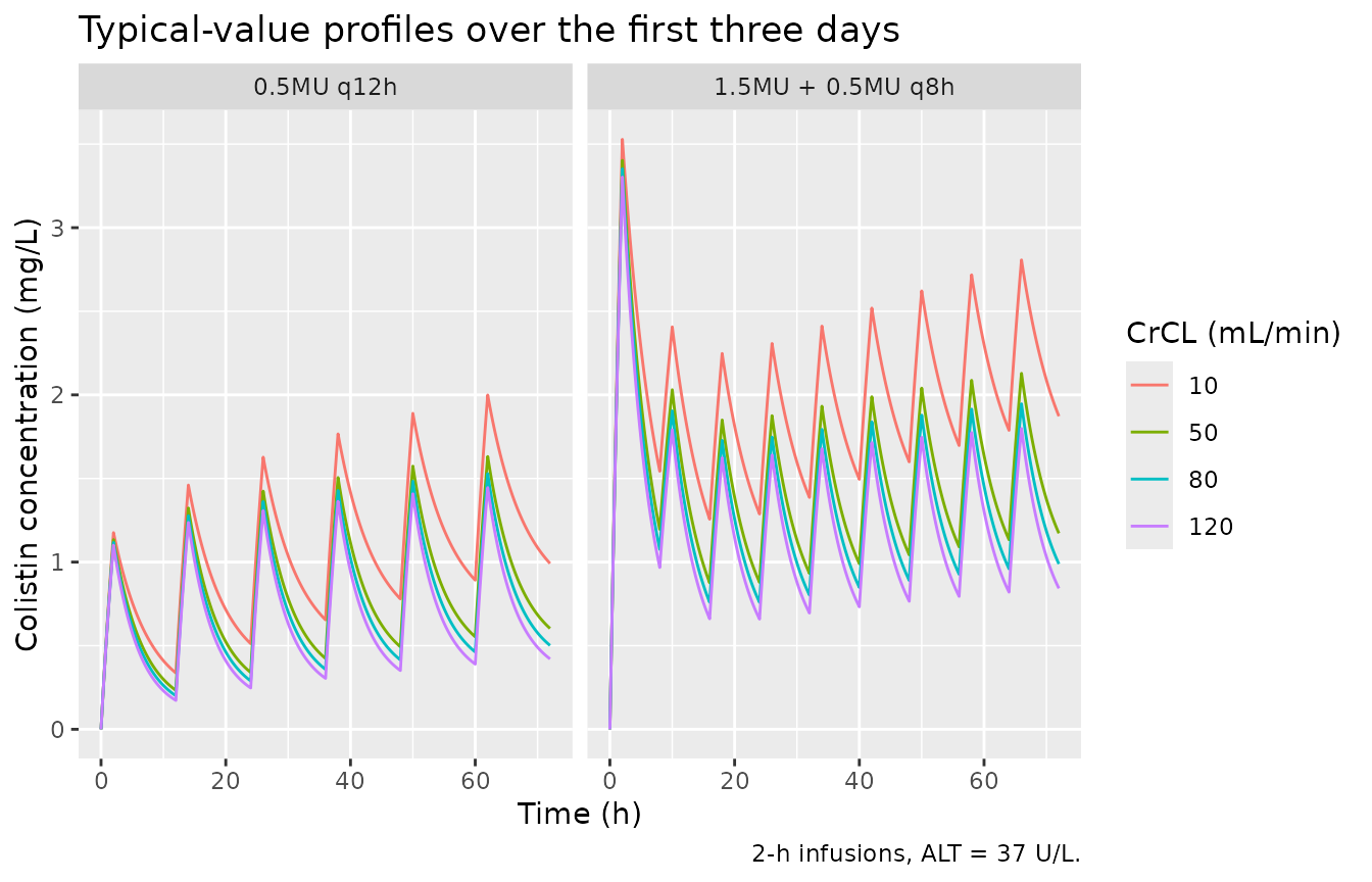
The ALT effect on V2 is large across the observed ALT range: V2 is 17.5 L at 7 U/L, 50.5 L at 37 U/L and 262 L at 495 U/L. Because V2 carries no elimination, it changes the time to reach steady state but not the steady-state average concentration.
PKNCA validation
nca_conc <- bind_rows(
  sim_course |> mutate(window = "course"),
  sim_ss |> mutate(window = "ss")
) |>
  filter(!is.na(Cc)) |>
  mutate(Cc = pmax(Cc, 0), treatment = paste0(regimen, " | CrCL ", CRCL)) |>
  select(id, time, Cc, treatment, regimen, CRCL)

dose_df <- bind_rows(events_course, events_ss) |>
  filter(evid == 1) |>
  mutate(treatment = paste0(regimen, " | CrCL ", CRCL)) |>
  select(id, time, amt, treatment)

conc_obj <- PKNCA::PKNCAconc(nca_conc, Cc ~ time | treatment + id,
                             concu = "mg/L", timeu = "h")
dose_obj <- PKNCA::PKNCAdose(dose_df, amt ~ time | treatment + id, doseu = "mg")

course_trt <- unique(nca_conc$treatment[!grepl("steady state", nca_conc$treatment)])
ss_trt <- unique(nca_conc$treatment[grepl("steady state", nca_conc$treatment)])

intervals <- bind_rows(
  tibble::tibble(treatment = course_trt, start = 0, end = 24, auclast = TRUE, cmax = TRUE),
  tibble::tibble(treatment = course_trt, start = 48, end = 72, auclast = TRUE, cmax = TRUE),
  tibble::tibble(treatment = ss_trt, start = 0, end = 12, auclast = TRUE, cmax = TRUE)
) |>
  as.data.frame()

nca_res <- PKNCA::pk.nca(PKNCA::PKNCAdata(conc_obj, dose_obj, intervals = intervals))
nca_df <- as.data.frame(nca_res)
stopifnot(nrow(nca_df) > 0)

auc_wide <- nca_df |>
  filter(PPTESTCD == "auclast") |>
  mutate(window = case_when(
    grepl("steady state", treatment) ~ "ss",
    start == 0 ~ "day1",
    TRUE ~ "day3"
  )) |>
  select(id, treatment, window, auc = PPORRES) |>
  left_join(distinct(nca_conc, id, regimen, CRCL), by = "id")

auc_wide |>
  group_by(Window = window, Regimen = regimen, `CrCL (mL/min)` = CRCL) |>
  summarise(`Median AUC (mg*h/L)` = median(auc), .groups = "drop") |>
  knitr::kable(digits = 1, caption = paste(
    "Simulated median AUC by window: day 1 (0-24 h), day 3 (48-72 h) and one",
    "steady-state 12-h interval."
))| Window | Regimen | CrCL (mL/min) | Median AUC (mg*h/L) |
|---|---|---|---|
| day1 | 0.5MU q12h | 10 | 17.6 |
| day1 | 0.5MU q12h | 50 | 14.9 |
| day1 | 0.5MU q12h | 80 | 13.7 |
| day1 | 0.5MU q12h | 120 | 12.9 |
| day1 | 1.5MU + 0.5MU q8h | 10 | 45.7 |
| day1 | 1.5MU + 0.5MU q8h | 50 | 37.0 |
| day1 | 1.5MU + 0.5MU q8h | 80 | 35.4 |
| day1 | 1.5MU + 0.5MU q8h | 120 | 33.0 |
| day3 | 0.5MU q12h | 10 | 31.3 |
| day3 | 0.5MU q12h | 50 | 23.0 |
| day3 | 0.5MU q12h | 80 | 20.1 |
| day3 | 0.5MU q12h | 120 | 18.5 |
| day3 | 1.5MU + 0.5MU q8h | 10 | 52.5 |
| day3 | 1.5MU + 0.5MU q8h | 50 | 36.1 |
| day3 | 1.5MU + 0.5MU q8h | 80 | 33.8 |
| day3 | 1.5MU + 0.5MU q8h | 120 | 29.9 |
| ss | 0.5MU q12h (steady state) | 10 | 25.9 |
| ss | 0.5MU q12h (steady state) | 50 | 15.3 |
| ss | 0.5MU q12h (steady state) | 80 | 13.3 |
| ss | 0.5MU q12h (steady state) | 120 | 11.7 |
Steady-state identity
At steady state AUC0-tau = Dose / CL exactly, for the
same drawn clearance. Both sides use each subject’s own CL, so the
difference is numerical error (trapezoidal integration over 0.25-h steps
and the ODE tolerances).
per_subject <- sim_ss |>
  group_by(id) |>
  summarise(cl = first(cl), .groups = "drop")

ss_check <- auc_wide |>
  filter(window == "ss") |>
  left_join(per_subject, by = "id") |>
  mutate(pct = 100 * (auc - 0.5 * mg_per_mu / cl) / (0.5 * mg_per_mu / cl))

tibble::tibble(
  `Median % difference` = median(ss_check$pct),
  `Max abs % difference` = max(abs(ss_check$pct))
) |>
knitr::kable(digits = 3, caption = "AUC0-12,ss versus Dose / CL, per subject.")| Median % difference | Max abs % difference |
|---|---|
| -0.003 | 0.057 |
Comparison against the published dosing simulations
Table 3 – probability of Css,avg above 2 and 4 mg/L
With Css,avg = daily dose / (24 * CL) and log-normal CL,
the model gives each Table 3 cell in closed form. The steady-state
cohort above checks the closed form for the 0.5 MU q12h row.
cl_typ <- function(crcl) 1.50 * (crcl / 57.5)^0.353
omega_cl <- sqrt(0.197)

table3_cmp <- table3_long |>
  mutate(
    model_pct = 100 * pnorm(log(daily_mu * mg_per_mu / (24 * cl_typ(CRCL)) / thr) / omega_cl),
    diff_pp = model_pct - pct
  )

table3_cmp |>
  filter(thr == 2) |>
  select(regimen, CRCL, Paper = pct, Model = model_pct) |>
  tidyr::pivot_wider(names_from = CRCL, values_from = c(Paper, Model)) |>
  knitr::kable(digits = 1, caption = paste(
    "P(Css,avg > 2 mg/L), percent: Xie 2022 Table 3 against the packaged",
    "model at true steady state. Columns are CrCL in mL/min."
))| regimen | Paper_10 | Paper_50 | Paper_80 | Paper_120 | Model_10 | Model_50 | Model_80 | Model_120 |
|---|---|---|---|---|---|---|---|---|
| 0.5MU q12h | 74.0 | 29.0 | 21.0 | 15.0 | 61.1 | 15.9 | 8.5 | 4.5 |
| 1.0MU + 0.5MU q12h | 85.5 | 37.5 | 28.0 | 17.0 | 61.1 | 15.9 | 8.5 | 4.5 |
| 1.5MU + 0.5MU q12h | 94.0 | 53.0 | 42.0 | 33.0 | 61.1 | 15.9 | 8.5 | 4.5 |
| 0.5MU q8h | 96.5 | 75.0 | 62.5 | 49.0 | 88.4 | 46.6 | 32.3 | 21.7 |
| 0.75MU q12h | 96.5 | 73.5 | 58.0 | 45.0 | 88.4 | 46.6 | 32.3 | 21.7 |
| 1.0MU + 0.5MU q8h | 98.0 | 77.0 | 69.5 | 56.5 | 88.4 | 46.6 | 32.3 | 21.7 |
| 1.0MU + 0.75MU q12h | 98.0 | 70.0 | 59.0 | 43.5 | 88.4 | 46.6 | 32.3 | 21.7 |
| 1.5MU + 0.5MU q8h | 98.5 | 82.0 | 68.5 | 57.0 | 88.4 | 46.6 | 32.3 | 21.7 |
| 1.5MU + 0.75MU q12h | 97.5 | 81.0 | 65.5 | 52.5 | 88.4 | 46.6 | 32.3 | 21.7 |
| 1.0 MU q12h | 99.5 | 88.5 | 78.0 | 69.0 | 96.7 | 71.3 | 57.5 | 44.7 |
| 1.5MU + 1.0 MU q12h | 100.0 | 87.0 | 79.5 | 71.5 | 96.7 | 71.3 | 57.5 | 44.7 |
| 1.0MU + 0.75MU q8h | 100.0 | 93.0 | 87.0 | 80.5 | 98.3 | 79.6 | 67.5 | 55.3 |
ss_sim_pct <- auc_wide |>
  filter(window == "ss") |>
  group_by(CRCL) |>
  summarise(sim_gt2 = 100 * mean(auc / 12 > 2), sim_median_css = median(auc / 12),
            .groups = "drop") |>
  mutate(closed_median_css = 0.5 * mg_per_mu / 12 / cl_typ(CRCL),
         closed_gt2 = 100 * pnorm(log(closed_median_css / 2) / omega_cl))

ss_sim_pct |>
  knitr::kable(digits = 2, caption = paste(
    "0.5 MU q12h at steady state: simulated cohort against the closed form."
))| CRCL | sim_gt2 | sim_median_css | closed_median_css | closed_gt2 |
|---|---|---|---|---|
| 10 | 59.0 | 2.16 | 2.27 | 61.09 |
| 50 | 14.0 | 1.27 | 1.28 | 15.90 |
| 80 | 10.0 | 1.11 | 1.09 | 8.50 |
| 120 | 4.5 | 0.97 | 0.94 | 4.51 |
# Cohort-derived. Median of 200 log-normal draws with SD 0.444 has a standard
# error of about 4%, so 12% is three standard errors; a mis-transcribed CL,
# exponent or dose conversion moves it by tens of percent.
stopifnot(
  all(abs(ss_sim_pct$sim_median_css / ss_sim_pct$closed_median_css - 1) < 0.12),
  # Binomial SE at n = 200 is at most 3.5 percentage points.
  all(abs(ss_sim_pct$sim_gt2 - ss_sim_pct$closed_gt2) < 12)
)
The packaged model reproduces the ranking and the
spread of Table 3 but not its level.
The paper’s probabilities are systematically higher. Inverting each
maintenance-only cell gives the median Css,avg implied by the paper,
which can be set against the model’s dose / CL:
level <- informative |>
  mutate(
    implied_median = thr * exp(z * omega_cl),
    model_median = daily_mu * mg_per_mu / (24 * cl_typ(CRCL)),
    ratio = implied_median / model_median
  ) |>
  group_by(`CrCL (mL/min)` = CRCL) |>
  summarise(`Paper-implied / model median Css,avg` = median(ratio),
            .groups = "drop")

knitr::kable(level, digits = 2, caption = paste(
  "Ratio of the median Css,avg implied by Xie 2022 Table 3 (maintenance-only",
  "rows) to the packaged model's typical value."
))| CrCL (mL/min) | Paper-implied / model median Css,avg |
|---|---|
| 10 | 1.19 |
| 50 | 1.28 |
| 80 | 1.30 |
| 120 | 1.32 |
# Deterministic arithmetic on printed numbers. This pins the documented
# discrepancy: a change to CL or its CrCL exponent moves these ratios.
stopifnot(all(level[[2]] > 1.05), all(level[[2]] < 1.45))
The paper’s simulated exposures exceed the model’s by about 20-30%, more at higher CrCL, which corresponds to a shallower CrCL effect than the published exponent of 0.353. Table 3 also changes with the loading dose (0.5 MU q12h alone versus with a 1.0 or 1.5 MU loading dose), which a true steady-state average cannot do, so the paper’s “Css,avg” was evaluated over a window before steady state. The text does not give that window. The packaged parameters are the published final estimates, identical in Table 2 and in Eqs 1-3, and they have not been adjusted to match the dosing tables. See “Assumptions and deviations”.
Figure 4 / Table S2 – probability of target attainment on day 3
The target is fAUC/MIC >= 20 with an unbound fraction
of 0.49 (Methods, “Monte Carlo simulation”), evaluated here on the day-3
AUC (48-72 h) and the day-1 AUC (0-24 h).
s2 <- tibble::tribble(
  ~regimen, ~day, ~MIC, ~`10`, ~`50`, ~`80`, ~`120`,
  "0.5MU q12h", "day1", 0.5, 31.5, 9.5, 5.5, 3,
  "0.5MU q12h", "day1", 1, 0, 0, 0, 0,
  "0.5MU q12h", "day1", 2, 0, 0, 0, 0,
  "0.5MU q12h", "day3", 0.5, 99, 91.5, 87.5, 77,
  "0.5MU q12h", "day3", 1, 89.5, 41.5, 31.5, 24,
  "0.5MU q12h", "day3", 2, 15.5, 1.5, 0, 0,
  "1.5MU + 0.5MU q8h", "day1", 0.5, 100, 99, 98.5, 95.5,
  "1.5MU + 0.5MU q8h", "day1", 1, 88, 46.5, 34.5, 19.5,
  "1.5MU + 0.5MU q8h", "day1", 2, 0, 0, 0, 0,
  "1.5MU + 0.5MU q8h", "day3", 0.5, 100, 98.5, 98.5, 96.5,
  "1.5MU + 0.5MU q8h", "day3", 1, 98.5, 87, 81.5, 69.5,
  "1.5MU + 0.5MU q8h", "day3", 2, 80, 36, 22.5, 16.5
) |>
  tidyr::pivot_longer(c(`10`, `50`, `80`, `120`), names_to = "CRCL",
                      values_to = "paper_pta") |>
  mutate(CRCL = as.numeric(CRCL))

pta_sim <- auc_wide |>
  filter(window %in% c("day1", "day3")) |>
  tidyr::crossing(MIC = c(0.5, 1, 2)) |>
  group_by(regimen, day = window, MIC, CRCL) |>
  summarise(model_pta = 100 * mean(0.49 * auc / MIC >= 20), .groups = "drop")

pta_cmp <- left_join(s2, pta_sim, by = c("regimen", "day", "MIC", "CRCL"))
stopifnot(!anyNA(pta_cmp$model_pta))

pta_cmp |>
  filter(day == "day3") |>
  tidyr::pivot_longer(c(paper_pta, model_pta), names_to = "source",
                      values_to = "PTA") |>
  mutate(source = ifelse(source == "paper_pta", "Xie 2022 (Table S2)", "Model")) |>
  ggplot(aes(CRCL, PTA, colour = factor(MIC), linetype = source)) +
  geom_line() +
  geom_point() +
  geom_hline(yintercept = 90, linetype = "dotted") +
  facet_wrap(~regimen) +
  labs(x = "CrCL (mL/min)", y = "PTA on day 3 (%)", colour = "MIC (mg/L)",
       linetype = NULL,
       caption = "Replicates Figure 4 of Xie 2022 (values from Supplementary Table S2).")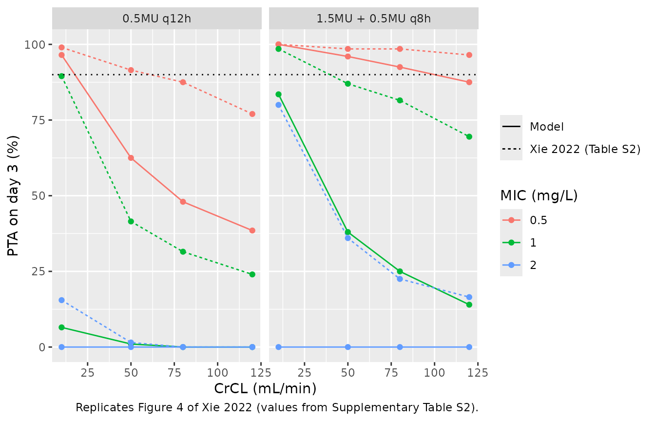
pta_cmp |>
  select(regimen, day, MIC, CRCL, `Paper PTA (%)` = paper_pta,
         `Model PTA (%)` = model_pta) |>
  knitr::kable(digits = 1, caption = paste(
    "Day-1 and day-3 PTA for fAUC/MIC >= 20 (f = 0.49): Xie 2022",
    "Supplementary Table S2 against the packaged model."
))| regimen | day | MIC | CRCL | Paper PTA (%) | Model PTA (%) |
|---|---|---|---|---|---|
| 0.5MU q12h | day1 | 0.5 | 10 | 31.5 | 9.5 |
| 0.5MU q12h | day1 | 0.5 | 50 | 9.5 | 1.0 |
| 0.5MU q12h | day1 | 0.5 | 80 | 5.5 | 0.0 |
| 0.5MU q12h | day1 | 0.5 | 120 | 3.0 | 0.0 |
| 0.5MU q12h | day1 | 1.0 | 10 | 0.0 | 0.0 |
| 0.5MU q12h | day1 | 1.0 | 50 | 0.0 | 0.0 |
| 0.5MU q12h | day1 | 1.0 | 80 | 0.0 | 0.0 |
| 0.5MU q12h | day1 | 1.0 | 120 | 0.0 | 0.0 |
| 0.5MU q12h | day1 | 2.0 | 10 | 0.0 | 0.0 |
| 0.5MU q12h | day1 | 2.0 | 50 | 0.0 | 0.0 |
| 0.5MU q12h | day1 | 2.0 | 80 | 0.0 | 0.0 |
| 0.5MU q12h | day1 | 2.0 | 120 | 0.0 | 0.0 |
| 0.5MU q12h | day3 | 0.5 | 10 | 99.0 | 96.5 |
| 0.5MU q12h | day3 | 0.5 | 50 | 91.5 | 62.5 |
| 0.5MU q12h | day3 | 0.5 | 80 | 87.5 | 48.0 |
| 0.5MU q12h | day3 | 0.5 | 120 | 77.0 | 38.5 |
| 0.5MU q12h | day3 | 1.0 | 10 | 89.5 | 6.5 |
| 0.5MU q12h | day3 | 1.0 | 50 | 41.5 | 1.0 |
| 0.5MU q12h | day3 | 1.0 | 80 | 31.5 | 0.0 |
| 0.5MU q12h | day3 | 1.0 | 120 | 24.0 | 0.0 |
| 0.5MU q12h | day3 | 2.0 | 10 | 15.5 | 0.0 |
| 0.5MU q12h | day3 | 2.0 | 50 | 1.5 | 0.0 |
| 0.5MU q12h | day3 | 2.0 | 80 | 0.0 | 0.0 |
| 0.5MU q12h | day3 | 2.0 | 120 | 0.0 | 0.0 |
| 1.5MU + 0.5MU q8h | day1 | 0.5 | 10 | 100.0 | 100.0 |
| 1.5MU + 0.5MU q8h | day1 | 0.5 | 50 | 99.0 | 99.0 |
| 1.5MU + 0.5MU q8h | day1 | 0.5 | 80 | 98.5 | 99.0 |
| 1.5MU + 0.5MU q8h | day1 | 0.5 | 120 | 95.5 | 94.5 |
| 1.5MU + 0.5MU q8h | day1 | 1.0 | 10 | 88.0 | 79.0 |
| 1.5MU + 0.5MU q8h | day1 | 1.0 | 50 | 46.5 | 31.5 |
| 1.5MU + 0.5MU q8h | day1 | 1.0 | 80 | 34.5 | 20.5 |
| 1.5MU + 0.5MU q8h | day1 | 1.0 | 120 | 19.5 | 11.5 |
| 1.5MU + 0.5MU q8h | day1 | 2.0 | 10 | 0.0 | 0.0 |
| 1.5MU + 0.5MU q8h | day1 | 2.0 | 50 | 0.0 | 0.0 |
| 1.5MU + 0.5MU q8h | day1 | 2.0 | 80 | 0.0 | 0.0 |
| 1.5MU + 0.5MU q8h | day1 | 2.0 | 120 | 0.0 | 0.0 |
| 1.5MU + 0.5MU q8h | day3 | 0.5 | 10 | 100.0 | 100.0 |
| 1.5MU + 0.5MU q8h | day3 | 0.5 | 50 | 98.5 | 96.0 |
| 1.5MU + 0.5MU q8h | day3 | 0.5 | 80 | 98.5 | 92.5 |
| 1.5MU + 0.5MU q8h | day3 | 0.5 | 120 | 96.5 | 87.5 |
| 1.5MU + 0.5MU q8h | day3 | 1.0 | 10 | 98.5 | 83.5 |
| 1.5MU + 0.5MU q8h | day3 | 1.0 | 50 | 87.0 | 38.0 |
| 1.5MU + 0.5MU q8h | day3 | 1.0 | 80 | 81.5 | 25.0 |
| 1.5MU + 0.5MU q8h | day3 | 1.0 | 120 | 69.5 | 14.0 |
| 1.5MU + 0.5MU q8h | day3 | 2.0 | 10 | 80.0 | 0.0 |
| 1.5MU + 0.5MU q8h | day3 | 2.0 | 50 | 36.0 | 0.0 |
| 1.5MU + 0.5MU q8h | day3 | 2.0 | 80 | 22.5 | 0.0 |
| 1.5MU + 0.5MU q8h | day3 | 2.0 | 120 | 16.5 | 0.0 |
The packaged model reproduces the qualitative conclusions of Figure 4 – PTA falls with rising CrCL and MIC, and the loading-dose regimen reaches the target earlier – but it predicts lower attainment than the paper. The gap is small on day 1 after the 1.5 MU loading dose, where exposure is set mainly by the dose and the volumes, and large on day 3 without a loading dose, where exposure depends on accumulation: at MIC 1 mg/L for 0.5 MU q12h at CrCL 10 mL/min, the paper gives 89.5% and the model about 7%. In the packaged two-compartment model the approach to steady state is slow (V2 = 50.5 L against CL2 = 1.71 L/h), so the paper’s simulations appear to accumulate faster than the printed parameters allow, as well as running at a higher level (Table 3 above).
# The paper's qualitative claims about Figure 4 that the model supports.
d3 <- pta_sim |> filter(day == "day3")
cell <- function(reg, mic, crcl) {
  d3$model_pta[d3$regimen == reg & d3$MIC == mic & d3$CRCL == crcl]
}
# Model-true values (3000 subjects per cell): 0.5 MU q12h at MIC 0.5 falls
# from 95% (CrCL 10) to 37% (CrCL 120); the loading-dose q8h regimen at MIC 1
# falls from 82% to 15% and exceeds 0.5 MU q12h (0-8%) by at least 15 points
# at every CrCL. The binomial SE at n = 200 is at most 3.5 points, so each
# bound below sits at least 3 SE inside the model-true difference.
stopifnot(
  # PTA falls as CrCL rises.
  cell("0.5MU q12h", 0.5, 10) > cell("0.5MU q12h", 0.5, 120) + 30,
  cell("1.5MU + 0.5MU q8h", 1, 10) > cell("1.5MU + 0.5MU q8h", 1, 120) + 30,
  # The loading-dose q8h regimen beats 0.5 MU q12h at every CrCL for MIC 1.
  all(vapply(crcl_grid, function(k) {
    cell("1.5MU + 0.5MU q8h", 1, k) > cell("0.5MU q12h", 1, k) + 5
  }, logical(1))),
  # At MIC 0.5 and severe renal impairment the target is met.
  cell("1.5MU + 0.5MU q8h", 0.5, 10) > 90
)
Supplementary Table S1 – urinary excretion
Urinary recovery (six patients) was analysed non-compartmentally and is not part of the model: median 10.05% of the dose recovered in 12 h and median renal clearance 0.209 L/h, 12.37% of total CL. The model’s typical CL at the cohort median CrCL of 48.8 mL/min is 1.42 L/h, so the paper’s renal fraction implies a non-renal clearance of roughly 1.21 L/h. The CrCL effect on CL therefore reflects more than glomerular filtration of colistin; the authors discuss extensive tubular reabsorption.
Assumptions and deviations
- Published dosing simulations not reproduced in level. Table 3, Figure 4 and Supplementary Table S2 show higher exposure than the published final parameters produce, by about 20-30% in median Css,avg, and the gap grows with CrCL. Their spread matches the published IIV, so the gap is in the typical clearance or its CrCL dependence used for the simulations. The printed parameters are internally consistent (Table 2 and Eqs 1-3 agree, and the bootstrap medians of 1.46 L/h and 0.373 are close to the estimates), so the model uses them as printed. Several simulation windows were tried (true steady state, day 3, day 1, cumulative 0-72 h, a one-compartment approximation) and none closes the gap. The paper’s Css,avg is not a true steady-state value, since it changes with the loading dose.
-
IIV scale. Table 2 labels the IIV rows
omega2and calls them variances; the Table 3 dose-ratio identity (omega about 0.35) sits nearer the variance reading (0.444) than the SD reading (0.197) and does not contradict it. -
Residual error. Phoenix NLME’s
stdev0for a proportional error model is the standard deviation of the proportional epsilon, sopropSd = 0.228. - Centring constants. CrCL is centred on 57.5 mL/min and ALT on 37 U/L, both taken from Eqs 2-3. The CrCL constant is not the Table 1 median (48.8 mL/min); the paper does not say which statistic it is.
- Renal replacement therapy. Two of 20 patients were on CRRT, with no separate treatment in the model; the model has no explicit dialysis clearance.
- Dose conversion. Doses are converted at the paper’s 10,000 IU = 0.44 mg (1 MU = 44 mg). The model itself is in mg and mg/L.
- ALT in simulations. The paper does not state the ALT used in its dosing simulations; this vignette uses the 37 U/L reference. ALT does not change the steady-state average concentration.
-
Screened covariates. Age, sex, weight, albumin and
the other laboratory variables listed in Methods were not retained; no
coefficients are reported. Age, sex, weight and albumin are documented
in
covariatesDataExcluded. - Exposure-response. The ROC analysis of clinical outcome against AUCss,0-24/MIC (Supplementary Figure S1) is descriptive and is not extracted.