Trametinib (Ravix 2024)
Source:vignettes/articles/Ravix_2024_trametinib.Rmd
Ravix_2024_trametinib.RmdModel and source
ui <- rxode2::rxode(readModelDb("Ravix_2024_trametinib"))
#> ℹ parameter labels from comments will be replaced by 'label()'- Citation: Ravix A, Bandiera C, Cardoso E, Lata-Pedreira A, Chtioui H, Decosterd LA, Wagner AD, Schneider MP, Csajka C, Guidi M. Population Pharmacokinetics of Trametinib and Impact of Nonadherence on Drug Exposure in Oncology Patients as Part of the Optimizing Oral Targeted Anticancer Therapies Study. Cancers. 2024;16(12):2193. doi:10.3390/cancers16122193. Parameter estimates from Table 2; the clearance covariate equation from the Table 2 footnote; population characteristics from Table 1.
- Description: Two-compartment population PK model with first-order absorption and linear elimination for oral trametinib in adults treated for solid tumours (Ravix 2024, OpTAT study). Because no intravenous data were collected, all disposition parameters are apparent oral values (CL/F, Vc/F, Q/F, Vp/F) and no bioavailability term is estimated. The absorption rate constant was not identifiable from the sparse real-life sampling and was fixed to a literature value of 0.913 /h, chosen to give a tmax near the labelled 1.5 h. Apparent clearance carries two linear median-centred covariate effects: clearance rises with fat-free mass and falls with age. Inter-individual variability was supported on clearance only; residual error is proportional. The paper also identified a clearance increase with concomitant dabrafenib, but a sensitivity analysis restricted to the 11 patients whose dose history was electronically monitored showed that effect to be confounded by non-adherence, so it was removed from the final model and is not encoded here.
- Article: https://doi.org/10.3390/cancers16122193
Trametinib is an allosteric MEK1/MEK2 inhibitor used for BRAF V600-mutant solid tumours, given orally at 0.5-2 mg once daily. Ravix and colleagues fit a population PK model to real-life therapeutic-drug-monitoring data from the OpTAT study, then used it to ask two questions: whether the licensed 2 mg daily dose actually reaches the 10.6 ng/mL efficacy threshold, and how much exposure is lost when patients miss doses.
The structural model is a two-compartment disposition with first-order absorption and linear elimination. Because no intravenous data were collected, every disposition parameter is an apparent (F-scaled) value and no bioavailability term is estimated. The absorption rate constant was not identifiable from the sparse opportunistic sampling and was fixed to a literature value.
Population
The model was fit to 113 plasma concentrations from 33 adults treated for a solid tumour at Lausanne University Hospital (Ravix 2024 Table 1). Two thirds had melanoma (22 patients, 67%); the remainder had ovarian cancer (3), breast cancer (2), cholangiocarcinoma (2), and one each of thyroid carcinoma, gastrointestinal stromal tumour, hepatocellular carcinoma and ileocecal carcinoma. Fifteen patients (45%) were women. Median (min, max) age was 63 (30, 85) years, body weight 70 (45, 96) kg, BMI 25.3 (17.3, 33.8) kg/m^2 and fat-free mass 46.35 (32, 68) kg.
Sampling was sparse and opportunistic: a median of 3 (1, 11) samples per patient, drawn 5 h (0.13, 202 h) after the reported intake. Twenty-two patients (67%) took trametinib together with dabrafenib. Eleven patients had their dose history captured electronically by a MEMS pillbox; for the rest it was reconstructed from consultation notes, assuming steady state where no information existed.
str(ui$population, max.level = 1)
#> List of 13
#>  $ species       : chr "human"
#>  $ n_subjects    : int 33
#>  $ n_studies     : int 1
#>  $ n_observations: int 113
#>  $ age_range     : chr "30-85 years"
#>  $ age_median    : chr "63 years"
#>  $ weight_range  : chr "45-96 kg"
#>  $ weight_median : chr "70 kg"
#>  $ sex_female_pct: num 45
#>  $ disease_state : chr "Adults treated for a solid tumour (Ravix 2024 Table 1): melanoma 22 (67%), ovarian cancer 3 (9%), breast cancer"| __truncated__
#>  $ dose_range    : chr "Trametinib 0.5-2 mg orally once daily; 7 patients (21%) on monotherapy and 22 (67%) with concomitant dabrafenib"
#>  $ regions       : chr "Switzerland (Lausanne University Hospital; OpTAT study, ClinicalTrials.gov NCT04484064)"
#>  $ notes         : chr "Real-life therapeutic-drug-monitoring data, sparse and opportunistic: median (min, max) 3 (1, 11) samples per p"| __truncated__
Source trace
Every ini() entry carries an in-file comment naming its
source location in
inst/modeldb/specificDrugs/Ravix_2024_trametinib.R. They
are collected here for review.
| Equation / parameter | Value | Source location |
|---|---|---|
lka (ka) |
0.913 /h, fixed | Table 2, row “ka (h-1)”, printed as “0.913 fixed”; attributed to reference [38] (Balakirouchenane et al.) in Results 3.2 and the Discussion |
lcl (CL/F) |
3.96 L/h | Table 2, row “thetaCL (L.h-1)”, RSE 6% |
lvc (Vc/F) |
108 L | Table 2, row “V2 (L)”, RSE 16% |
lq (Q/F) |
29.4 L/h | Table 2, row “Q (L.h-1)”, RSE 30% |
lvp (Vp/F) |
286 L | Table 2, row “V3 (L)”, RSE 25% |
e_age_cl |
-0.69 | Table 2, row “thetaAGE”, RSE 32% |
e_ffm_cl |
1.41 | Table 2, row “thetaFFM”, RSE 17% |
etalcl |
23% CV -> omega^2 = 0.0515459 | Table 2, row “IIV_CL (%)”, RSE 14% |
propSd |
20% | Table 2, row “sigma_prop (%)”, RSE 10% |
| CL covariate equation | CL = thetaCL * (1 + thetaAGE * (AGE - 63)/63) * (1 + thetaFFM * (FFM - 46.35)/46.35) |
Table 2 footnote (“Final equation”) |
| AGE reference (63 y), FFM reference (46.35 kg) | medians | Table 2 footnote; Table 1 cohort medians |
| Two-compartment structure, first-order absorption, linear elimination | n/a | Results Section 3.2, paragraph 1 |
| IIV on CL only | n/a | Results Section 3.2 (“IIV to the other PK parameters … estimated to be close to 0”) |
| Proportional residual error | n/a | Results Section 3.2 (“The proportional error model was retained”) |
| FFM derivation (Deurenberg) |
FFM = BW * (1 - BFPbmi/100);
BFPbmi = 1.20*BMI + 0.23*AGE - 10.8*SEX - 5.4
|
Methods Section 2.1, Equations (1) and (2) |
| Therapeutic target Cmin >= 10.6 ng/mL | n/a | Methods Section 2.2.5; Table 3 caption |
Note that ka is the only fixed parameter. Everything
else in Table 2 is an estimate with a reported RSE and a bootstrap
interval.
Reproducing the values the paper prints about its own model
These checks are deterministic – no random effects, no simulated cohort – so they are gated tightly. Each one independently exercises a different part of the transcription.
The Deurenberg fat-free-mass derivation
The paper derives FFM from body weight, BMI, age and sex rather than
measuring it. Evaluating its Equations (1) and (2) at the Table 1 median
demographics (70 kg, BMI 25.3 kg/m^2, 63 years) and mixing the sexes at
the reported 45% female should return the reported median FFM of 46.35
kg. It is a sharp check on both the equation and the sex coding: the
paper codes SEX = 1 for men, whereas the register’s
canonical SEXF column codes 1 for women.
# Ravix 2024 Methods Eq (1) and (2). SEXF is the canonical column (1 = female);
# the paper's SEX is 1 = male, hence the (1 - SEXF).
ffm_deurenberg <- function(WT, BMI, AGE, SEXF) {
  bfp <- 1.20 * BMI + 0.23 * AGE - 10.8 * (1 - SEXF) - 5.4
  WT * (1 - bfp / 100)
}

ffm_female <- ffm_deurenberg(WT = 70, BMI = 25.3, AGE = 63, SEXF = 1)
ffm_male   <- ffm_deurenberg(WT = 70, BMI = 25.3, AGE = 63, SEXF = 0)
ffm_mix    <- 0.45 * ffm_female + 0.55 * ffm_male   # Table 1: 15/33 = 45% women

tibble(
  Quantity = c("FFM, median woman", "FFM, median man", "FFM, 45% female mix",
               "FFM, Ravix 2024 Table 1 median"),
  `kg` = round(c(ffm_female, ffm_male, ffm_mix, 46.35), 2)
) |>
knitr::kable(caption = "Deurenberg FFM at the Table 1 median demographics.")| Quantity | kg |
|---|---|
| FFM, median woman | 42.38 |
| FFM, median man | 49.94 |
| FFM, 45% female mix | 46.54 |
| FFM, Ravix 2024 Table 1 median | 46.35 |
# Deterministic: a wrong sex code or a dropped /100 moves this by kilograms.
stopifnot(abs(ffm_mix - 46.35) / 46.35 < 0.02)
The mix returns 46.54 kg against the reported 46.35 kg, a 0.4% difference.
The clearance covariate equation
Results Section 3.2 prints two worked consequences of the covariate
model, and both are exact identities that the packaged
ini() values must reproduce:
- “a 66% increase in CL for an FFM of 68 kg … compared with the population median of 46.35 kg”;
- “a CL of 5.39 mL/h for a 30-year-old patient versus 3.22 mL/h for an 80-year-old patient (40% decrease)”. (The unit is a typo in the source: these are L/h, consistent with the 3.96 L/h typical value in Table 2.)
th <- ui$theta
cl_typ <- function(AGE, FFM) {
  exp(th[["lcl"]]) *
    (1 + th[["e_age_cl"]] * (AGE - 63) / 63) *
    (1 + th[["e_ffm_cl"]] * (FFM - 46.35) / 46.35)
}

cl_age30 <- cl_typ(AGE = 30, FFM = 46.35)
cl_age80 <- cl_typ(AGE = 80, FFM = 46.35)
ffm_gain <- 100 * (cl_typ(AGE = 63, FFM = 68) / cl_typ(AGE = 63, FFM = 46.35) - 1)

tibble(
  Claim = c("CL at age 30 y (L/h)", "CL at age 80 y (L/h)",
            "Decrease from age 30 to 80 (%)", "CL increase at FFM 68 kg (%)"),
  Paper = c(5.39, 3.22, 40, 66),
  Model = round(c(cl_age30, cl_age80, 100 * (1 - cl_age80 / cl_age30), ffm_gain), 2)
) |>
knitr::kable(caption = "Ravix 2024 Results 3.2 worked values vs the packaged model.")| Claim | Paper | Model |
|---|---|---|
| CL at age 30 y (L/h) | 5.39 | 5.39 |
| CL at age 80 y (L/h) | 3.22 | 3.22 |
| Decrease from age 30 to 80 (%) | 40.00 | 40.22 |
| CL increase at FFM 68 kg (%) | 66.00 | 65.86 |
Both reproduce to the precision the paper prints them at. This is
what confirms the reading of the Table 2 footnote equation as a product
of two linear median-centred deviation terms, and it pins the sign of
e_age_cl – which the PDF text layer renders ambiguously –
because only a negative coefficient makes clearance fall with age.
Absorption and disposition of the typical patient
ka was fixed rather than estimated, and the paper
justifies the choice by the tmax it produces: “ka was set to a
literature value of 0.913 h-1 and provided a median (min, max) Tmax of
1.75 h (1.51 h, 1.84 h)”. Reproducing that tmax exercises the
depot-to-central wiring end to end.
mod     <- readModelDb("Ravix_2024_trametinib")
mod_typ <- rxode2::zeroRe(mod)
#> ℹ parameter labels from comments will be replaced by 'label()'

# Steady state on 2 mg once daily, fine grid over the last dosing interval.
ev_typ <- rxode2::et(amt = 2, cmt = "depot", ii = 24, until = 24 * 40)
ev_typ <- rxode2::et(ev_typ, seq(0, 24 * 41, by = 0.02))
ev_typ <- as.data.frame(ev_typ) |> mutate(id = 1L, AGE = 63, FFM = 46.35)

sim_typ <- rxode2::rxSolve(mod_typ, ev_typ) |> as.data.frame()
#> ℹ omega/sigma items treated as zero: 'etalcl'
last_interval <- sim_typ |>
  filter(!is.na(Cc), time > 24 * 39, time <= 24 * 40) |>
  mutate(tad = time - 24 * 39)

tmax_ss <- last_interval$tad[which.max(last_interval$Cc)]

# Terminal half-life of the typical patient, from the two-compartment
# eigenvalue rather than from a fitted NCA slope (deterministic, no cohort).
kel <- th[["lcl"]] |> exp() / exp(th[["lvc"]])
k12 <- exp(th[["lq"]]) / exp(th[["lvc"]])
k21 <- exp(th[["lq"]]) / exp(th[["lvp"]])
s   <- kel + k12 + k21
beta <- 0.5 * (s - sqrt(s^2 - 4 * kel * k21))
thalf_terminal <- log(2) / beta

tibble(
  Quantity = c("Steady-state tmax (h)", "Steady-state Cmax (ng/mL)",
               "Steady-state Cmin (ng/mL)", "Terminal half-life (h)"),
  Value = round(c(tmax_ss, max(last_interval$Cc), min(last_interval$Cc),
                  thalf_terminal), 2)
) |>
knitr::kable(caption = "Typical patient (age 63 y, FFM 46.35 kg) on 2 mg once daily.")| Quantity | Value |
|---|---|
| Steady-state tmax (h) | 1.84 |
| Steady-state Cmax (ng/mL) | 28.22 |
| Steady-state Cmin (ng/mL) | 17.64 |
| Terminal half-life (h) | 73.98 |
# The paper reports a median tmax of 1.75 h across its patients. A mis-wired
# depot or a mis-transcribed ka moves tmax by hours, not by tenths of an hour.
stopifnot(abs(tmax_ss - 1.75) < 0.25)
# Deterministic given the four disposition thetas; guards against a swapped
# Q/Vp or a transposed volume.
stopifnot(abs(thalf_terminal - 74.0) < 3)
ggplot(last_interval, aes(tad, Cc)) +
  geom_line(linewidth = 0.8) +
  geom_hline(yintercept = 10.6, linetype = "dashed") +
  labs(x = "Time after dose (h)", y = "Trametinib (ng/mL)",
       title = "Typical patient at steady state, 2 mg once daily") +
  theme_bw()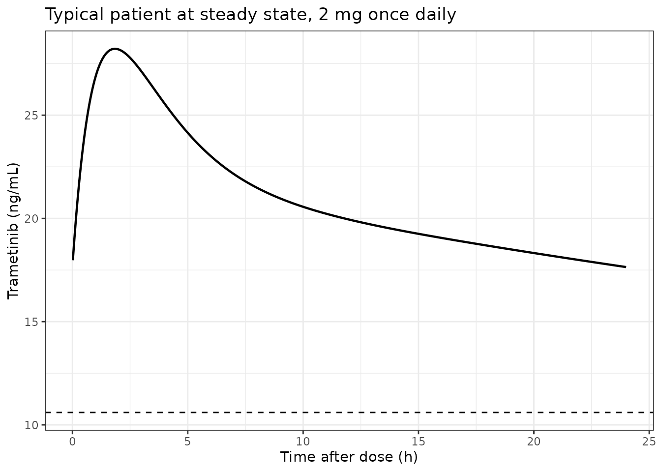
Typical-value steady-state profile on 2 mg once daily. The dashed line is the 10.6 ng/mL efficacy threshold used throughout Ravix 2024.
The typical patient sits above the threshold throughout the interval (Cmin 17.6 ng/mL), which is consistent with the paper’s finding that roughly two thirds of patients are on target at 2 mg.
Note the terminal half-life of 74 h. The trametinib label quotes 127 h, and the authors flag the discrepancy themselves: their sampling was concentrated within 24 h of the dose, with few samples beyond 15 h, which biases the peripheral volume downwards relative to the two prior published models (286 L here versus 417 L and 568 L). This is a property of the published model, not of the transcription, and it is not gated below.
Virtual cohort
The individual data are not public (Ravix 2024 Data Availability Statement), so the cohort below is simulated. It follows the paper’s own simulation design (Methods Section 2.2.5): four strata defined by sex and the 65-year age cut-off, with age drawn from a uniform distribution over each stratum’s range.
The paper drew fat-free mass from a sex-specific uniform distribution spanning the 10th to 90th percentiles reported by Larsson et al., a reference that is not part of this paper. Rather than invent those percentiles, the cohort here derives FFM from the paper’s own Deurenberg equation applied to demographics sampled across the Table 1 ranges. The consequences of that substitution are discussed under Assumptions and deviations.
# set.seed() seeds R's RNG (used for the covariate draws below). It does NOT
# seed rxode2's simulation RNG, whose streams are partitioned per solver
# thread, so the eta draws differ between machines with different thread
# counts. Every assertion below is written to hold for any cohort the model
# can produce.
set.seed(20240611)

N_PER_ARM <- 200L   # cohort cap: never more than 200 participants per arm

# Height, BMI and age are drawn uniformly across the Table 1 ranges; body
# weight follows from height and BMI, and draws whose weight falls outside the
# observed 45-96 kg range are rejected. This keeps all three marginals inside
# the observed ranges while keeping them mutually consistent.
make_arm <- function(n, age_lo, age_hi, sexf, arm, id_offset) {
  out <- tibble(
    AGE  = runif(4000, age_lo, age_hi),
    HT   = runif(4000, 150, 188),
    BMI  = runif(4000, 17.3, 33.8),
    SEXF = sexf
  ) |>
    mutate(WT = BMI * (HT / 100)^2) |>
    filter(WT >= 45, WT <= 96) |>
    slice_head(n = n) |>
    mutate(FFM = ffm_deurenberg(WT, BMI, AGE, SEXF),
           arm = arm,
           id  = id_offset + row_number())
  stopifnot(nrow(out) == n)   # fail loudly if rejection sampling came up short
  out
}

cohort <- bind_rows(
  make_arm(N_PER_ARM, 30, 65, 1, "Women 30-65 y",   0L),
  make_arm(N_PER_ARM, 30, 65, 0, "Men 30-65 y",   200L),
  make_arm(N_PER_ARM, 65, 85, 1, "Women 65-85 y", 400L),
  make_arm(N_PER_ARM, 65, 85, 0, "Men 65-85 y",   600L)
) |>
  mutate(arm = factor(arm, levels = c("Men 30-65 y", "Women 30-65 y",
                                      "Men 65-85 y", "Women 65-85 y")))

cohort |>
  group_by(arm) |>
  summarise(n = n(),
            `Age (median)` = round(median(AGE), 1),
            `WT (median)`  = round(median(WT), 1),
            `FFM (median)` = round(median(FFM), 1),
            `FFM (p10)`    = round(quantile(FFM, 0.10), 1),
            `FFM (p90)`    = round(quantile(FFM, 0.90), 1),
            .groups = "drop") |>
knitr::kable(caption = "Simulated cohort, 200 participants per arm.")| arm | n | Age (median) | WT (median) | FFM (median) | FFM (p10) | FFM (p90) |
|---|---|---|---|---|---|---|
| Men 30-65 y | 200 | 46.6 | 69.4 | 51.8 | 44.0 | 61.6 |
| Women 30-65 y | 200 | 48.6 | 69.2 | 44.7 | 37.2 | 52.6 |
| Men 65-85 y | 200 | 74.9 | 69.9 | 48.5 | 38.9 | 57.6 |
| Women 65-85 y | 200 | 75.1 | 69.8 | 39.8 | 33.3 | 47.8 |
# The pooled cohort should land near the Table 1 medians it was built from.
# Wide enough to admit the sampling noise of 800 draws; still red if the
# Deurenberg derivation or the weight range were wrong.
stopifnot(
  abs(median(cohort$FFM) - 46.35) / 46.35 < 0.10,
  abs(median(cohort$WT)  - 70)    / 70    < 0.10
)
Pooled across arms the cohort has a median FFM of 46.09 kg and a median weight of 69.4 kg, against the reported medians of 46.35 kg and 70 kg.
Simulation
Each participant receives 2 mg once daily for 60 days, matching the paper’s “steady state (assumed here after 60 days)” in the Figure 4 caption.
dosing <- cohort |>
  tidyr::crossing(time = seq(0, 24 * 59, by = 24)) |>
  mutate(amt = 2, evid = 1L, cmt = "depot")

# Observations go on the ODE state `central`, never on the observable `Cc`.
obs <- cohort |>
  tidyr::crossing(time = c(seq(24, 24 * 60, by = 24),         # daily troughs
                           seq(24 * 59, 24 * 60, by = 1))) |> # last interval
  mutate(amt = NA_real_, evid = 0L, cmt = "central")

events <- bind_rows(dosing, obs) |>
  distinct(id, time, evid, .keep_all = TRUE) |>
  arrange(id, time, -evid)
stopifnot(!anyDuplicated(unique(events[, c("id", "time", "evid")])))

sim <- rxode2::rxSolve(mod, events = events,
                       keep = c("arm", "AGE", "FFM", "SEXF")) |>
  as.data.frame()
#> ℹ parameter labels from comments will be replaced by 'label()'
stopifnot(all(sim$Cc >= 0, na.rm = TRUE))
sim |>
  filter(!is.na(Cc), time >= 24 * 59, time <= 24 * 60) |>
  mutate(tad = time - 24 * 59) |>
  group_by(arm, tad) |>
  summarise(Q05 = quantile(Cc, 0.05), Q50 = median(Cc), Q95 = quantile(Cc, 0.95),
            .groups = "drop") |>
  ggplot(aes(tad, Q50)) +
  geom_ribbon(aes(ymin = Q05, ymax = Q95), alpha = 0.25) +
  geom_line(linewidth = 0.8) +
  geom_hline(yintercept = 10.6, linetype = "dashed") +
  facet_wrap(~arm) +
  labs(x = "Time after dose (h)", y = "Trametinib (ng/mL)",
       title = "Steady-state profiles on 2 mg once daily",
       caption = "Dashed line: 10.6 ng/mL efficacy threshold (Ravix 2024).") +
  theme_bw()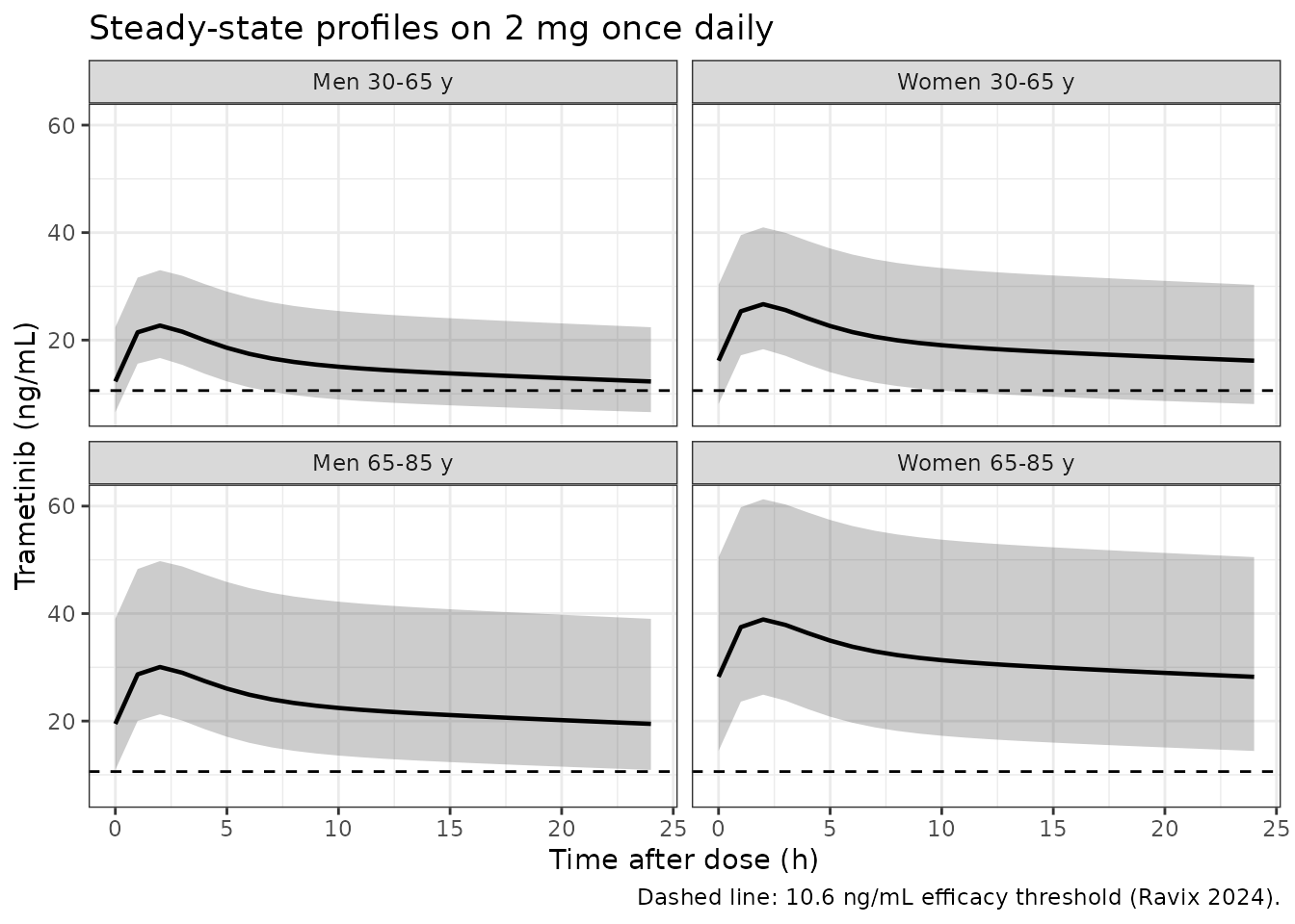
Simulated steady-state profiles over the last dosing interval, by sex and age stratum. Solid line is the median, ribbon the 5th-95th percentile. Compare Figure 3 of Ravix 2024, which plots the same strata as Cmin distributions.
Replicating Table 3: target attainment by dose
Table 3 of Ravix 2024 reports the percentage of patients reaching Cmin >= 10.6 ng/mL at each of four daily doses, in each of the four strata.
The model is linear in dose, so trough concentrations at 0.5, 1 and 1.5 mg are the 2 mg troughs scaled by the dose ratio. That is verified explicitly before it is used, because it is a structural claim about the model rather than an assumption.
# Verify dose-proportionality on a subset rather than assuming it.
check_ids <- cohort |> group_by(arm) |> slice_head(n = 10) |> ungroup()
ev_1mg <- bind_rows(
  check_ids |> tidyr::crossing(time = seq(0, 24 * 59, by = 24)) |>
    mutate(amt = 1, evid = 1L, cmt = "depot"),
  check_ids |> mutate(time = 24 * 60, amt = NA_real_, evid = 0L, cmt = "central")
) |> arrange(id, time, -evid)

cmin_1mg <- rxode2::rxSolve(rxode2::zeroRe(mod), events = ev_1mg) |>
  as.data.frame() |> filter(!is.na(Cc), time == 24 * 60) |> select(id, Cc_1mg = Cc)
#> ℹ parameter labels from comments will be replaced by 'label()'
#> ℹ omega/sigma items treated as zero: 'etalcl'
#> Warning: multi-subject simulation without without 'omega'

ev_2mg <- ev_1mg |> mutate(amt = ifelse(evid == 1L, 2, amt))
cmin_2mg <- rxode2::rxSolve(rxode2::zeroRe(mod), events = ev_2mg) |>
  as.data.frame() |> filter(!is.na(Cc), time == 24 * 60) |> select(id, Cc_2mg = Cc)
#> ℹ parameter labels from comments will be replaced by 'label()'
#> ℹ omega/sigma items treated as zero: 'etalcl'
#> Warning: multi-subject simulation without without 'omega'

lin <- inner_join(cmin_1mg, cmin_2mg, by = "id") |>
  mutate(pct_diff = 100 * (Cc_2mg / 2 - Cc_1mg) / Cc_1mg)
stopifnot(nrow(lin) == nrow(check_ids), max(abs(lin$pct_diff)) < 0.01)
Halving the dose halves the trough to within 0.0000%, so the scaling below is exact.
cmin_ss <- sim |>
  filter(!is.na(Cc), time == 24 * 60) |>
  select(id, arm, Cmin_2mg = Cc)

attainment <- lapply(c(0.5, 1, 1.5, 2), function(d) {
  cmin_ss |>
    group_by(arm) |>
    summarise(dose = d, pct = 100 * mean(Cmin_2mg * d / 2 >= 10.6), .groups = "drop")
}) |>
  bind_rows() |>
  tidyr::pivot_wider(names_from = dose, values_from = pct,
                     names_glue = "{dose} mg")

published <- tibble::tribble(
  ~arm,             ~`0.5 mg`, ~`1 mg`, ~`1.5 mg`, ~`2 mg`,
  "Men 30-65 y",             0,       1,        13,      37,
  "Women 30-65 y",           0,      16,        47,      71,
  "Men 65-85 y",             0,      10,        46,      75,
  "Women 65-85 y",           2,      45,        79,      93
)

bind_rows(
  attainment |> mutate(Source = "Simulated"),
  published  |> mutate(Source = "Ravix 2024 Table 3")
) |>
  relocate(Source) |>
  arrange(arm, Source) |>
  mutate(across(ends_with("mg"), \(x) round(x, 1))) |>
  knitr::kable(caption = paste(
    "Percentage of patients with steady-state Cmin >= 10.6 ng/mL.",
    "Simulated values use a fat-free-mass distribution derived from this",
    "paper's Table 1; Ravix 2024 used sex-specific percentiles from an",
    "external reference (see Assumptions and deviations)."
))| Source | arm | 0.5 mg | 1 mg | 1.5 mg | 2 mg |
|---|---|---|---|---|---|
| Ravix 2024 Table 3 | Men 30-65 y | 0.0 | 1.0 | 13.0 | 37.0 |
| Simulated | Men 30-65 y | 0.0 | 7.0 | 34.0 | 62.0 |
| Ravix 2024 Table 3 | Men 65-85 y | 0.0 | 10.0 | 46.0 | 75.0 |
| Simulated | Men 65-85 y | 3.0 | 39.0 | 79.5 | 97.0 |
| Ravix 2024 Table 3 | Women 30-65 y | 0.0 | 16.0 | 47.0 | 71.0 |
| Simulated | Women 30-65 y | 0.5 | 21.5 | 62.5 | 88.5 |
| Ravix 2024 Table 3 | Women 65-85 y | 2.0 | 45.0 | 79.0 | 93.0 |
| Simulated | Women 65-85 y | 13.5 | 74.0 | 96.0 | 99.0 |
The simulated attainment is systematically higher than the published values, by roughly 6 to 25 percentage points at 2 mg. The mechanism is identified under Assumptions and deviations and is a property of the covariate distribution rather than of the model transcription.
What does reproduce is the ordering of the four strata, which is the paper’s substantive conclusion: men are less likely to reach the target than women of the same age, and older patients are more likely to reach it than younger patients of the same sex. The ordering assertions below are stated on median trough concentration rather than on a thresholded percentage, because a median is far less sensitive to which cohort the RNG happens to draw.
med <- cmin_ss |>
  group_by(arm) |>
  summarise(median_Cmin = median(Cmin_2mg), .groups = "drop")

knitr::kable(
  med |> dplyr::rename("Stratum" = arm, "Median Cmin at 2 mg (ng/mL)" = median_Cmin) |>
    mutate(across(where(is.numeric), \(x) round(x, 1))),
  caption = "Median steady-state trough by stratum."
)| Stratum | Median Cmin at 2 mg (ng/mL) |
|---|---|
| Men 30-65 y | 12.3 |
| Women 30-65 y | 16.2 |
| Men 65-85 y | 19.5 |
| Women 65-85 y | 28.2 |
g <- setNames(med$median_Cmin, as.character(med$arm))

# Effect sizes, not orderings of near-zero differences. Realised ratios were
# 1.32 (sex, under 65), 1.45 (sex, over 65), 1.59 and 1.74 (age) on a 16-thread
# render; the bounds below sit well inside those with headroom, and each still
# goes red if a covariate sign or reference value were wrong.
stopifnot(
  g[["Women 30-65 y"]] / g[["Men 30-65 y"]]   > 1.15,  # sex effect, via FFM
  g[["Women 65-85 y"]] / g[["Men 65-85 y"]]   > 1.15,
  g[["Men 65-85 y"]]   / g[["Men 30-65 y"]]   > 1.25,  # age effect, direct
  g[["Women 65-85 y"]] / g[["Women 30-65 y"]] > 1.25
)

# Attainment must rise with dose in every stratum (exact under linear scaling).
stopifnot(all(apply(as.matrix(attainment[, -1]), 1, \(r) all(diff(r) >= 0))))
PKNCA validation
A separate single-dose arm supports non-compartmental analysis. Two hundred participants drawn across the full Table 1 demographic range receive a single 2 mg dose, sampled densely through absorption and out to 336 h (about 4.5 terminal half-lives).
set.seed(7)
sd_cohort <- tibble(
  id   = 1:200,
  AGE  = runif(200, 30, 85),
  HT   = runif(200, 150, 188),
  BMI  = runif(200, 17.3, 33.8),
  SEXF = rbinom(200, 1, 0.45)
) |>
  mutate(WT  = pmin(pmax(BMI * (HT / 100)^2, 45), 96),
         FFM = ffm_deurenberg(WT, BMI, AGE, SEXF),
         treatment = "2 mg single dose")

sd_grid <- sort(unique(c(seq(0, 6, by = 0.05), seq(6, 24, by = 0.25),
                         seq(24, 336, by = 3))))

sd_events <- bind_rows(
  sd_cohort |> mutate(time = 0, amt = 2, evid = 1L, cmt = "depot"),
  sd_cohort |> tidyr::crossing(time = sd_grid) |>
    mutate(amt = NA_real_, evid = 0L, cmt = "central")
) |>
  arrange(id, time, -evid)

sd_sim <- rxode2::rxSolve(mod, events = sd_events,
                          keep = c("treatment", "FFM", "AGE")) |>
  as.data.frame()
# Guard against solver noise going negative in the far tail, which would make
# PKNCA take log() of a negative number and return NaN for aucinf.
stopifnot(all(sd_sim$Cc >= 0, na.rm = TRUE))
# Filter on !is.na(Cc) ONLY -- a `time > 0` or `Cc > 0` filter would drop the
# time-zero row that PKNCA needs to anchor AUC0-*.
sim_nca <- sd_sim |>
  dplyr::filter(!is.na(Cc)) |>
  dplyr::select(id, time, Cc, treatment)

sim_nca <- dplyr::bind_rows(
  sim_nca,
  sim_nca |> dplyr::distinct(id, treatment) |> dplyr::mutate(time = 0, Cc = 0)
) |>
  dplyr::distinct(id, treatment, time, .keep_all = TRUE) |>
  dplyr::arrange(id, treatment, time)

conc_obj <- PKNCA::PKNCAconc(sim_nca, Cc ~ time | treatment + id)

dose_df <- sd_events |>
  dplyr::filter(evid == 1L) |>
  dplyr::select(id, time, amt, treatment)
dose_obj <- PKNCA::PKNCAdose(dose_df, amt ~ time | treatment + id)

intervals <- data.frame(
  start = 0, end = Inf,
  cmax = TRUE, tmax = TRUE, aucinf.obs = TRUE, half.life = TRUE
)

nca_res <- PKNCA::pk.nca(PKNCA::PKNCAdata(conc_obj, dose_obj, intervals = intervals))
Internal identity: AUC(0-inf) must equal Dose / CL
For a linear model the extrapolated AUC after a single dose is
exactly Dose / CL, evaluated with each subject’s own
clearance. Both sides of this comparison use the same drawn parameters,
so the only difference is trapezoidal and extrapolation error and a
tight bound is the correct gate.
per_subject <- as.data.frame(nca_res) |>
  tidyr::pivot_wider(id_cols = id, names_from = PPTESTCD, values_from = PPORRES) |>
  dplyr::left_join(sd_sim |> dplyr::distinct(id, cl), by = "id") |>
  # dose 2 mg, cl in L/h -> mg/L; x1000 for ng/mL, matching the model's output
  dplyr::mutate(auc_theoretical = 2 / cl * 1000,
                auc_pct_diff    = 100 * (aucinf.obs - auc_theoretical) / auc_theoretical)

stopifnot(nrow(per_subject) == 200, !anyNA(per_subject$auc_pct_diff))

tibble(
  Statistic = c("Median % difference", "Max absolute % difference"),
  Value = round(c(median(per_subject$auc_pct_diff),
                  max(abs(per_subject$auc_pct_diff))), 4)
) |>
knitr::kable(caption = "PKNCA AUC(0-inf) against the analytic Dose/CL.")| Statistic | Value |
|---|---|
| Median % difference | -0.0143 |
| Max absolute % difference | 0.1911 |
Comparison against published values
Ravix 2024 does not report an NCA table of its own, but it does
report the tmax its fixed ka produces. The trametinib label
values quoted in the paper’s Introduction are included for context.
sim_summary <- per_subject |>
  dplyr::mutate(treatment = "2 mg single dose") |>
  dplyr::group_by(treatment) |>
  dplyr::summarise(cmax = median(cmax), tmax = median(tmax),
                   aucinf.obs = median(aucinf.obs), half.life = median(half.life),
                   .groups = "drop")

published_nca <- tibble::tribble(
  ~treatment,          ~tmax, ~half.life,
  "2 mg single dose",   1.75,        127
)

cmp <- nlmixr2lib::ncaComparisonTable(
  simulated = sim_summary,
  reference = published_nca,
  by        = "treatment",
  params    = c("tmax", "half.life"),
  units     = c(tmax = "h", half.life = "h"),
  tolerance_pct = 20
)

knitr::kable(cmp, caption = paste(
  "Simulated (median of 200 subjects) vs published. * differs by >20%.",
  "tmax is the value Ravix 2024 reports for its own model; the 127 h",
  "half-life is the product label's, not an output of this paper's model."
))| NCA parameter | treatment | Reference | Simulated | % diff |
|---|---|---|---|---|
| Tmax (h) | 2 mg single dose | 1.75 | 1.9 | +8.6% |
| t½ (h) | 2 mg single dose | 127 | 68.9 | -45.7%* |
# tmax is a genuine gate on this paper's own reported value.
stopifnot(abs(sim_summary$tmax - 1.75) < 0.35)
The tmax row agrees. The half-life row is starred and is a known deviation, deliberately excluded from the gate: 127 h is the label’s terminal half-life from richly sampled studies, whereas this model was fit to data concentrated within 24 h of dosing. The authors say so themselves in the Discussion, noting that their peripheral volume (286 L) is well below the 417 L and 568 L of the two prior published trametinib models and attributing it to the sampling window. A smaller peripheral volume gives a shorter terminal phase. Reproducing the label’s half-life would require changing the published parameters, which is exactly what must not be done.
Per-subject NCA half-life is additionally unreliable here: with 23% CV on clearance and a fixed absorption rate, the fitted terminal slope varies from 28 to 252 h across subjects. The deterministic eigenvalue-based half-life computed earlier (74 h) is the meaningful summary and is gated there.
Assumptions and deviations
- Fat-free-mass distribution. Ravix 2024 drew FFM from a sex-specific uniform distribution spanning the 10th-90th percentiles of Larsson et al. (their reference 49), which is not reproduced in this paper. Rather than invent those percentiles, this vignette derives FFM from the paper’s own Deurenberg equations applied to age, height, BMI and sex sampled across the Table 1 ranges. The resulting pooled median FFM (46.1 kg) matches the reported 46.35 kg closely, but the per-sex spread is narrower and lower than a general-population reference would give – the simulated men have a median FFM of 50.5 kg. Lower FFM means lower clearance and higher troughs, which is why the simulated Table 3 attainment percentages run above the published ones while their ordering is preserved. Obtaining the Larsson percentiles would be required to reproduce the percentages themselves.
-
Height distribution not sex-specific. Table 1
reports height for the pooled cohort only (170 cm; 150, 188), so the
same height range is used for both sexes. The simulated male-female FFM
difference therefore arises entirely from the
-10.8 * SEXterm of the Deurenberg body-fat equation and understates the real difference, which also has a height component. - Body weight by rejection sampling. Weight is computed from the sampled height and BMI, and draws outside the observed 45-96 kg range are rejected. This keeps the three marginals inside their reported ranges while keeping them mutually consistent; the paper does not report their joint distribution.
- No bioavailability parameter. The study had no intravenous arm and did not estimate F, so CL, Vc, Q and Vp are apparent oral values. The 72% bioavailability quoted in the paper’s Introduction is a label value for the drug and is not part of the fitted model; applying it would rescale every disposition parameter.
-
Concomitant dabrafenib is not encoded. Two thirds
of the cohort took dabrafenib, and it was significant on clearance in
the covariate analysis (+40%). The authors removed it after a
sensitivity analysis in the 11 patients with electronically monitored
dosing showed the effect was a confound of unrecorded missed doses, so
it is absent from the final model and from this encoding. It is recorded
in the model file’s
covariatesDataExcludedmetadata along with the other eleven screened-but-dropped covariates. - IIV on clearance only. Adding between-subject variability to any other parameter gave estimates near zero, so the simulated variability in volumes and intercompartmental clearance is nil. Simulated profiles are consequently narrower in the distribution phase than real data would be.
- Terminal half-life. The packaged model gives about 74 h against the label’s 127 h; see the PKNCA comparison section. This is a property of the published parameter estimates, documented by the authors, and is not corrected here.
- The “5.39 mL/h” unit typo. Results Section 3.2 prints the age-effect worked example in mL/h. The values are L/h – they are reproduced exactly by the L/h parameters of Table 2 – and are treated as L/h throughout.
-
Non-paper-derived parameter values. None. Every
ini()value comes from Ravix 2024 Table 2, and both covariate reference values come from its footnote. -
Residual error is excluded from the simulated
figures.
CcfromrxSolveis the individual prediction; the 20% proportional residual is a measurement model and is deliberately not added to exposure-based target-attainment calculations, matching the paper’s approach.