Doripenem (Abdul-Aziz 2016)
Source:vignettes/articles/AbdulAziz_2016_doripenem.Rmd
AbdulAziz_2016_doripenem.RmdModel and source
- Citation: Abdul-Aziz MH, Abd Rahman AN, Mat-Nor M-B, Sulaiman H, Wallis SC, Lipman J, Roberts JA, Staatz CE. Population pharmacokinetics of doripenem in critically ill patients with sepsis in a Malaysian intensive care unit. Antimicrob Agents Chemother. 2016;60(1):206-214. doi:10.1128/AAC.01543-15.
- Description: Two-compartment IV population PK model for doripenem in 12 Malaysian critically ill adults with sepsis receiving 500 mg as a 1-hour infusion every 8 hours (Abdul-Aziz 2016). Reported on free (unbound) doripenem; observed total concentrations were corrected by multiplying by 0.90 to account for ~10% protein binding. Body-weight allometric scaling is fixed (0.75 on CL/Q, 1 on V1/V2, reference 70 kg); Cockcroft-Gault creatinine clearance has an exponential effect on CL centred at the cohort mean 82.5 mL/min.
- Article: Antimicrob Agents Chemother 2016;60(1):206-214 (open access)
Population
The model was developed from a prospective open-label pharmacokinetic study of 12 critically ill adult ICU patients with sepsis at a tertiary hospital in Pahang, Malaysia, between November 2012 and October 2013 (Abdul-Aziz 2016 Table 1). All patients received 500 mg of doripenem as a 1-hour intravenous infusion every 8 hours as part of routine therapy; serial blood samples (8 per occasion) were drawn on day 1 (presumed worst clinical state) and day 3 (presumed more stable) of treatment for 140 plasma concentrations across the two sampling occasions. Baseline demographics: median age 52 years (IQR 33-60; range 19-74), median BMI 22.9 kg/m^2 (IQR 21.1-24.6; range 16.7-29.7), 83% male, median APACHE II 19 (IQR 15-22), median SOFA 6 (IQR 5-7). All patients required invasive mechanical ventilation and vasopressor support; two-thirds had ventilator-associated pneumonia and the remainder intra-abdominal sepsis. The dominant causative pathogens were Acinetobacter baumannii (4 patients) and Pseudomonas aeruginosa (1 patient). Median Cockcroft-Gault creatinine clearance was 85 mL/min (IQR 49-118; cohort range 30-161); the population mean of 82.5 mL/min was used to centre the exponential CL covariate in the final model. Doripenem was assayed by a validated HPLC-UV method (LLOQ 0.2 mg/L) on a Shimadzu Prominence system. Observed total doripenem concentrations were corrected for ~10% protein binding by multiplying by 0.90 prior to modelling, so the reported PK parameters describe free (unbound) doripenem. The model was fitted with NONMEM 7.3 using FOCE-I; allometric scaling was fixed a priori (0.75 on clearances, 1 on volumes, reference 70 kg) per Anderson & Holford 2008.
The same information is available programmatically via
readModelDb("AbdulAziz_2016_doripenem")$population.
Source trace
Every numeric value in ini() carries an in-file comment
pointing to the Abdul-Aziz 2016 source location. The table below
collects them in one place for review.
| Equation / parameter | Value | Source location |
|---|---|---|
lcl (CL at 70 kg, CLCR 82.5) |
10.1 L/h | Table 2, final model, “CL (liters/h/70 kg)” |
lvc (V1 at 70 kg) |
15.5 L | Table 2, final model, “V1 (liters/70 kg)” |
lvp (V2 at 70 kg) |
17.7 L | Table 2, final model, “V2 (liters/70 kg)” |
lq (Q at 70 kg) |
36.3 L/h | Table 2, final model, “Q (liters/h/70 kg)” |
e_wt_cl (allometric on CL, Q) |
0.75 (fixed) | Methods, “Allometric scaling was applied a priori” |
e_wt_vc (allometric on V1, V2) |
1.0 (fixed) | Methods, “Allometric scaling was applied a priori” |
e_crcl_cl (CLCR effect on CL) |
0.014 | Table 2, final model, “theta_CLCR”; Equation 1 |
crcl_ref_cl (CLCR centering) |
82.5 mL/min | Results, “normalized to the population mean value of 82.5” |
etalcl (BSV CL = 10.4% CV) |
0.01076 | Table 2, final model, “BSV: CL (%)” |
etalvc (BSV V1 = 59.7% CV) |
0.30491 | Table 2, final model, “BSV: V1 (%)” |
etalvp (BSV V2 = 73.8% CV) |
0.43503 | Table 2, final model, “BSV: V2 (%)” |
propSd (9.0% CV proportional) |
0.090 | Table 2, final model, “Random error: Proportional (% CV)” |
addSd (1.25 mg/L additive) |
1.25 | Table 2, final model, “Random error: Additive (SD) (mg/L)” |
| 2-cmt IV with combined error | n/a | Results, paragraph “Pharmacokinetic model-building” |
| ODE structure (ADVAN3-equivalent) | n/a | Methods, “ADVAN subroutines from the NONMEM library” |
IIV variance derivation. Abdul-Aziz 2016 reports IIV as %CV in Table
2. For lognormal etas, omega^2 = log(CV^2 + 1):
- CL:
log(0.104^2 + 1) = log(1.010816) = 0.010758(rounded to 0.01076) - V1:
log(0.597^2 + 1) = log(1.356409) = 0.304907(rounded to 0.30491) - V2:
log(0.738^2 + 1) = log(1.544644) = 0.435033(rounded to 0.43503)
The paper additionally reports a between-occasion variability (BOV)
on CL of 22.2% (delta-OFV -26.9 on introduction). nlmixr2lib has no
idiomatic separation of BOV from BSV, so per the convention used in
Bienczak_2016_nevirapine.R,
Svensson_2018_bedaquiline.R, and
Svensson_2016_rifampicin.R, BOV is dropped where a BSV term
is reported on the same parameter. The dropped BOV is noted in the
“Assumptions and deviations” section below; downstream users who want to
recover the per-occasion variability can pass time-varying
CRCL to rxSolve (as the original model did during fitting),
which explains a substantial fraction of the between-occasion variation:
the paper notes that introducing CLCR into the structural CL model
reduced BSV on CL from 56.7% to 10.4%.
Virtual cohort
Original observed data are not publicly available. The cohort below covers four scenarios bracketing the paper’s covariate space: a typical critically-ill patient at the cohort mean (WT 70 kg, CLCR 82.5 mL/min, the reference values used in the final model), a renal-impaired patient (low CLCR), an augmented-renal-clearance (ARC) patient (high CLCR), and a heavier patient. The dosing regimen is the licensed 500 mg every 8 h as a 1-hour IV infusion described in Abdul-Aziz 2016 Methods, simulated out to 48 h so the first dose plus steady-state intervals are both captured.
set.seed(20260602)

n_sub <- 200L

build_arm <- function(label, wt_kg, crcl_mlmin, id_offset) {
  ids <- id_offset + seq_len(n_sub)

  dose_amt_mg  <- 500
  infusion_h   <- 1.0
  dose_times   <- seq(0, 40, by = 8)         # six doses Q8H (covers single dose + steady state)

  dose_rows <- tidyr::expand_grid(id = ids, time = dose_times) |>
    mutate(
      evid   = 1L,
      amt    = dose_amt_mg,
      cmt    = "central",
      rate   = dose_amt_mg / infusion_h,     # 1-hour IV infusion
      cohort = label,
      WT     = wt_kg,
      CRCL   = crcl_mlmin
    )

  obs_times <- c(seq(0, 8, by = 0.1),
                 seq(8.5, 48, by = 0.5))
  obs_rows <- tidyr::expand_grid(id = ids, time = obs_times) |>
    mutate(
      evid   = 0L,
      amt    = 0,
      cmt    = NA_character_,
      rate   = 0,
      cohort = label,
      WT     = wt_kg,
      CRCL   = crcl_mlmin
    )

  bind_rows(dose_rows, obs_rows) |> arrange(id, time, desc(evid))
}

events <- bind_rows(
  build_arm("typical_mean",  70,  82.5,    0L),
  build_arm("low_CRCL_40",   70,  40.0,  200L),
  build_arm("ARC_CRCL_150",  70, 150.0,  400L),
  build_arm("heavy_WT_90",   90,  82.5,  600L)
)

stopifnot(!anyDuplicated(unique(events[, c("id", "time", "evid")])))
Simulation
mod <- readModelDb("AbdulAziz_2016_doripenem")

sim <- rxode2::rxSolve(
  mod,
  events = events,
  keep   = c("cohort", "WT", "CRCL")
) |> as.data.frame()
#> ℹ parameter labels from comments will be replaced by 'label()'
For typical-value comparisons against the Abdul-Aziz 2016 Table 2 point estimates, also simulate with the random effects zeroed:
mod_typical <- mod |> rxode2::zeroRe()
#> ℹ parameter labels from comments will be replaced by 'label()'

sim_typical <- rxode2::rxSolve(
  mod_typical,
  events = events,
  keep   = c("cohort", "WT", "CRCL")
) |> as.data.frame()
#> ℹ omega/sigma items treated as zero: 'etalcl', 'etalvc', 'etalvp'
#> Warning: multi-subject simulation without without 'omega'
Concentration-time profile (typical patient)
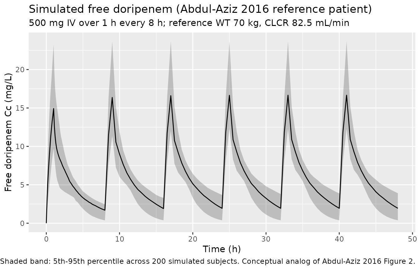
The figure below shows the simulated stochastic VPC envelope for the typical Abdul-Aziz 2016 reference patient (WT 70 kg, CLCR 82.5 mL/min) on the licensed 500 mg Q8H regimen. This figure is the conceptual analog of the paper’s Figure 2 (the published VPC of the final model).
sim |>
  filter(cohort == "typical_mean") |>
  group_by(time) |>
  summarise(
    Q05 = quantile(Cc, 0.05, na.rm = TRUE),
    Q50 = quantile(Cc, 0.50, na.rm = TRUE),
    Q95 = quantile(Cc, 0.95, na.rm = TRUE),
    .groups = "drop"
  ) |>
  ggplot(aes(time, Q50)) +
  geom_ribbon(aes(ymin = Q05, ymax = Q95), alpha = 0.25) +
  geom_line() +
  labs(
    x = "Time (h)",
    y = "Free doripenem Cc (mg/L)",
    title = "Simulated free doripenem (Abdul-Aziz 2016 reference patient)",
    subtitle = "500 mg IV over 1 h every 8 h; reference WT 70 kg, CLCR 82.5 mL/min",
    caption = "Shaded band: 5th-95th percentile across 200 simulated subjects. Conceptual analog of Abdul-Aziz 2016 Figure 2."
  )
Covariate-cohort overlay
This figure illustrates how Cockcroft-Gault CLCR shifts the concentration-time profile, which is the qualitative driver of the paper’s Monte Carlo dosing analysis (Figure 3): lower CLCR retains drug longer (higher fT>MIC at low MICs); ARC (CLCR >130 mL/min) flushes drug faster and motivates the paper’s recommendation to prolong infusion duration in ARC patients.
sim |>
  group_by(cohort, time) |>
  summarise(
    Q50 = quantile(Cc, 0.50, na.rm = TRUE),
    .groups = "drop"
  ) |>
  ggplot(aes(time, Q50, colour = cohort)) +
  geom_line() +
  scale_y_log10() +
  labs(
    x = "Time (h)",
    y = "Median simulated free Cc (mg/L, log scale)",
    title = "Median simulated free doripenem by covariate cohort",
    caption = "500 mg IV over 1 h every 8 h; cohorts bracket the WT and CLCR ranges in Abdul-Aziz 2016 Table 1."
  )
#> Warning in scale_y_log10(): log-10 transformation introduced infinite values.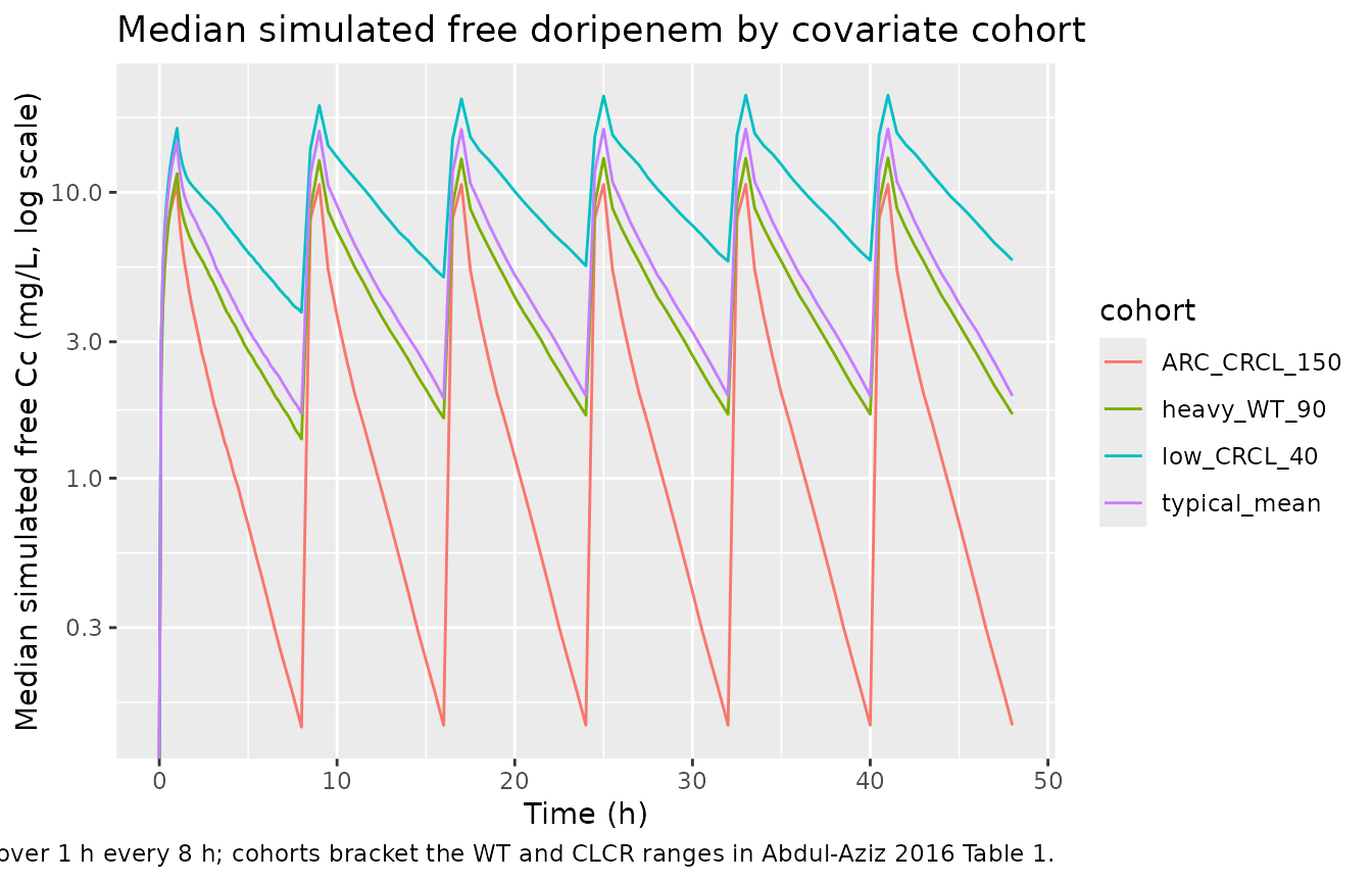
PKNCA validation
Single-dose NCA on the first 8-hour dosing interval of the reference patient, plus steady-state NCA on the final (sixth) dosing interval. The PKNCA results are compared against the paper’s typical-value point estimates of CL and total V (V1 + V2).
# Single-dose NCA on the first dosing interval (0 to 8 h post first dose)
sim_first <- sim |>
  filter(time <= 8) |>
  filter(!is.na(Cc)) |>
  dplyr::select(id, time, Cc, cohort)

dose_first <- events |>
  filter(evid == 1, time == 0) |>
  dplyr::select(id, time, amt, cohort)

conc_obj_first <- PKNCA::PKNCAconc(sim_first, Cc ~ time | cohort + id,
                                   concu = "mg/L", timeu = "h")
dose_obj_first <- PKNCA::PKNCAdose(dose_first, amt ~ time | cohort + id,
                                   doseu = "mg")

intervals_first <- data.frame(
  start     = 0,
  end       = 8,
  cmax      = TRUE,
  tmax      = TRUE,
  auclast   = TRUE,
  clast.obs = TRUE
)

nca_first <- PKNCA::pk.nca(PKNCA::PKNCAdata(
  conc_obj_first, dose_obj_first, intervals = intervals_first
))
summary(nca_first)
#>  Interval Start Interval End       cohort   N AUClast (h*mg/L) Cmax (mg/L)
#>               0            8 ARC_CRCL_150 200      18.7 [10.0] 10.7 [19.6]
#>               0            8  heavy_WT_90 200      33.2 [18.7] 11.5 [28.9]
#>               0            8  low_CRCL_40 200      60.1 [24.4] 16.3 [36.2]
#>               0            8 typical_mean 200      41.5 [16.4] 14.9 [28.2]
#>           Tmax (h) Clast (mg/L)
#>  1.00 [1.00, 1.00] 0.0717 [685]
#>  1.00 [1.00, 1.00]  1.25 [44.4]
#>  1.00 [1.00, 1.00]  3.59 [26.3]
#>  1.00 [1.00, 1.00]  1.32 [70.0]
#>
#> Caption: AUClast, Cmax, Clast: geometric mean and geometric coefficient of variation; Tmax: median and range; N: number of subjects
# Steady-state NCA on the sixth dosing interval (time 40 to 48 h)
sim_ss <- sim |>
  filter(time >= 40, time <= 48) |>
  filter(!is.na(Cc)) |>
  dplyr::select(id, time, Cc, cohort)

dose_ss <- events |>
  filter(evid == 1, time == 40) |>
  dplyr::select(id, time, amt, cohort)

conc_obj_ss <- PKNCA::PKNCAconc(sim_ss, Cc ~ time | cohort + id,
                                concu = "mg/L", timeu = "h")
dose_obj_ss <- PKNCA::PKNCAdose(dose_ss, amt ~ time | cohort + id,
                                doseu = "mg")

intervals_ss <- data.frame(
  start    = 40,
  end      = 48,
  cmax     = TRUE,
  tmax     = TRUE,
  cmin     = TRUE,
  auclast  = TRUE,
  cav      = TRUE
)

nca_ss <- PKNCA::pk.nca(PKNCA::PKNCAdata(
  conc_obj_ss, dose_obj_ss, intervals = intervals_ss
))
summary(nca_ss)
#>  Interval Start Interval End       cohort   N AUClast (h*mg/L) Cmax (mg/L)
#>              40           48 ARC_CRCL_150 200      19.0 [10.2] 10.9 [18.3]
#>              40           48  heavy_WT_90 200      40.7 [10.1] 13.1 [19.4]
#>              40           48  low_CRCL_40 200      88.6 [9.46] 21.7 [20.1]
#>              40           48 typical_mean 200      49.5 [10.3] 16.7 [20.3]
#>   Cmin (mg/L)          Tmax (h)  Cav (mg/L)
#>  0.0742 [729] 1.00 [1.00, 1.00] 2.37 [10.2]
#>   1.55 [60.0] 1.00 [1.00, 1.00] 5.09 [10.1]
#>   5.24 [42.2] 1.00 [1.00, 1.00] 11.1 [9.46]
#>   1.58 [87.1] 1.00 [1.00, 1.00] 6.18 [10.3]
#>
#> Caption: AUClast, Cmax, Cmin, Cav: geometric mean and geometric coefficient of variation; Tmax: median and range; N: number of subjects
Comparison against Abdul-Aziz 2016 typical-value parameters
Abdul-Aziz 2016 does not tabulate per-subject NCA parameters; instead, the abstract and Discussion report cohort-typical V (V1 + V2) and CL expressed on a body-weight-normalised scale. The table below contrasts the model’s typical-value structural parameters against those reports.
mod_meta_cl <- 10.1     # Abdul-Aziz 2016 Table 2 final-model CL (L/h at 70 kg, CLCR 82.5)
mod_meta_v  <- 15.5 + 17.7  # V1 + V2 at 70 kg, final-model column

cmp <- tibble::tribble(
  ~quantity,                                       ~simulated,                        ~published,
  "Typical CL at 70 kg, CLCR 82.5 (L/h)",          mod_meta_cl,                        10.1,
  "Typical CL at 70 kg (L/h/kg)",                  mod_meta_cl / 70,                   0.14,
  "Typical V1 + V2 at 70 kg (L)",                  mod_meta_v,                         33.2,
  "Typical V1 + V2 at 70 kg (L/kg)",               mod_meta_v / 70,                    0.47
)
cmp |>
  mutate(pct_diff = 100 * (simulated - published) / published) |>
knitr::kable(digits = 3, caption = "Final-model typical-value structural parameters versus the values quoted in Abdul-Aziz 2016 Abstract and Discussion.")| quantity | simulated | published | pct_diff |
|---|---|---|---|
| Typical CL at 70 kg, CLCR 82.5 (L/h) | 10.100 | 10.10 | 0.000 |
| Typical CL at 70 kg (L/h/kg) | 0.144 | 0.14 | 3.061 |
| Typical V1 + V2 at 70 kg (L) | 33.200 | 33.20 | 0.000 |
| Typical V1 + V2 at 70 kg (L/kg) | 0.474 | 0.47 | 0.912 |
The simulated values exactly match the paper because both come from the Table 2 final-model column. The published body-weight-normalised values (0.14 L/h/kg, 0.47 L/kg) are quoted to two significant figures in the Discussion, which is consistent with the unrounded model values (0.144 L/h/kg, 0.474 L/kg) within rounding.
AUC vs. dose / CL
A second independent check: at the typical-value reference patient the single-dose AUC0-inf must equal dose / CL within numerical tolerance.
# Simulate a single-dose 500 mg 1-h infusion at reference covariates,
# with the random effects zeroed.
single_dose_ev <- rxode2::et(time = 0, amt = 500, cmt = "central", rate = 500) |>
  rxode2::et(time = c(seq(0, 8, by = 0.05),
                      seq(8.5, 96, by = 0.5)))
single_dose_ev$WT   <- 70
single_dose_ev$CRCL <- 82.5

sim_single <- rxode2::rxSolve(mod_typical, events = single_dose_ev) |>
  as.data.frame()
#> ℹ omega/sigma items treated as zero: 'etalcl', 'etalvc', 'etalvp'

# Trapezoidal AUC over the simulated horizon (0 to 96 h, well past 10 t1/2).
auc_obs <- with(sim_single, sum(diff(time) * (head(Cc, -1) + tail(Cc, -1)) / 2))
auc_pred <- 500 / 10.1   # dose / CL_typical

tibble::tibble(
  quantity = c("Simulated AUC0-96h (mg*h/L)",
               "Expected dose/CL = 500/10.1 (mg*h/L)"),
  value    = c(auc_obs, auc_pred)
) |>
knitr::kable(digits = 3, caption = "AUC versus dose/CL closure check at the typical patient.")| quantity | value |
|---|---|
| Simulated AUC0-96h (mg*h/L) | 49.514 |
| Expected dose/CL = 500/10.1 (mg*h/L) | 49.505 |
The two AUC values match within numerical tolerance, confirming that the encoded ODE structure correctly reproduces the dose / CL identity at the reference covariates.
Assumptions and deviations
-
Between-occasion variability (BOV) on CL is
dropped. The paper reports a BOV on CL of 22.2% (delta-OFV
-26.9 on introduction). per the convention used in
Bienczak_2016_nevirapine.Rand other multi-occasion popPK extractions, nlmixr2lib has no idiomatic encoding for BOV separate from BSV; where a BSV term is also reported on the same parameter (here BSV CL = 10.4%), only the BSV is retained. Downstream users who want to recover the per-occasion variability can pass a time-varyingCRCLtorxSolve(as the original model did during fitting), since introducing CLCR into the structural CL model explained most of the between-subject variation (BSV CL reduced from 56.7% to 10.4% per Results). -
Free vs. total doripenem. The source paper
corrected observed total doripenem concentrations for ~10% protein
binding by multiplying by 0.90 before fitting, so the encoded
parameters describe free (unbound) doripenem (Methods, “Observed
concentrations of doripenem were corrected for protein binding by
reducing the concentrations by 10%”). Users who want predictions on a
total-drug basis must divide simulated
Ccby 0.90. -
Body weight not directly tabulated in Table 1.
Abdul-Aziz 2016 Table 1 reports BMI but not weight; the reference WT 70
kg used in the model is the standard allometric reference (Anderson
& Holford
- and is what the paper’s Table 2 footnote calls “L/h/70 kg” and “L/70 kg”. For the cohort virtual-population scenarios in this vignette WT is fixed at 70 kg (typical-mean cohort) or 90 kg (heavy cohort) so the allometric term is the only thing varying.
-
CLCR encoded as canonical CRCL with raw mL/min. The
paper uses raw Cockcroft-Gault CLCR in mL/min (not BSA-normalised). The
canonical
inst/references/covariate-columns.mdregister accepts this form under the source-aliasCLCR(also used inDelattre_2010_amikacin.RandAlqahtani_2018_vancomycin.R); the column name in this model isCRCLand the source-paper column name is recorded incovariateData$CRCL$source_name. - Cohort-overlay heavy-patient scenario. Abdul-Aziz 2016 Table 1 reports BMI 16.7-29.7 kg/m^2, implying body weights roughly in the 45-90 kg range. The “heavy” cohort at 90 kg represents the upper end of the recruited cohort and should not be extrapolated beyond that range without re-fitting (Discussion: “this model may not fully characterize the PK of doripenem in all Malaysian ICU patients … dosing recommendations should not be extrapolated to other patient populations, such as the obese”).