Lamivudine (Ojara 2024)
Source:vignettes/articles/Ojara_2024_lamivudine.Rmd
Ojara_2024_lamivudine.RmdModel and source
mod <- readModelDb("Ojara_2024_lamivudine")
ui <- rxode2::rxode(mod)
#> ℹ parameter labels from comments will be replaced by 'label()'- Citation: Ojara FW, Kawuma AN, Nakalema S, Kyohairwe I, Nakijoba R, Lamorde M, Pertinez H, Khoo S, Waitt C. Population pharmacokinetic modeling of paired plasma-breast milk lamivudine data for estimation of infant exposure in breastfeeding mother-infant pairs. CPT Pharmacometrics Syst Pharmacol. 2024;13(11):1978-1989. doi:10.1002/psp4.13274. Structural equations from Methods Equations 1-3; parameter estimates from Table 2.
- Description: Lactation population PK model for oral lamivudine in breastfeeding Ugandan women living with HIV, fitted simultaneously to paired maternal plasma and breast-milk concentrations across a full 24-hour dosing interval. First-order absorption without lag time into a one-compartment plasma disposition model; plasma-to-breast-milk transfer is a partitioned effect compartment whose concentration state equilibrates at first-order rate ke0 towards ppc times the plasma concentration, where ppc is the estimated milk-to-plasma concentration ratio of 1.77. That structure reproduces the observed lag between the plasma and breast-milk concentration peaks (2 h vs 6 h). Correlated exponential interindividual variability on clearance and central volume, independent interindividual variability on the milk-to-plasma ratio, no interindividual variability on absorption, and separate proportional residual errors for plasma and for breast milk. Clearance and volume are apparent oral values. No covariates were retained in the final model.
- Article: https://doi.org/10.1002/psp4.13274 (open access; PMC11578128)
This is the first lamivudine lactation population PK model. The
maternal plasma disposition is a one-compartment model with first-order
absorption; breast-milk transfer is a partitioned effect
compartment whose concentration state equilibrates at first-order
rate ke0 towards ppc times the plasma
concentration (Ojara 2024 Equation 3):
ppc (the paper’s Rcb) is therefore the
milk-to-plasma concentration ratio, and
ke0 (the paper’s Kcb) sets how fast that ratio
is approached, which is what produces the observed lag between the
plasma and the breast-milk concentration peaks.
Population
The model was fitted to an observational study of 35 Ugandan women living with HIV, recruited antenatally at the Infectious Diseases Institute in Kampala between 2016 and 2017 and sampled postpartum (Ojara 2024 Table 1). Ten mothers received lamivudine 150 mg twice daily with nevirapine and zidovudine; 25 received 300 mg once daily with efavirenz and tenofovir disoproxil fumarate. Maternal weight was 64.0 kg (50.0, 89.0), age 30 years (19, 40), BMI 24.8 kg/m^2 (20.0, 30.5), and Cockcroft-Gault creatinine clearance 134.6 mL/min (89.2, 184.7) – elevated, as is typical postpartum. Mothers attended two of three possible visits; visit 1 was 13.0 days (7.00, 43.0) postpartum and visit 2 was 73.5 days (36.0, 84.0). Infant weight was 3.60 kg (2.40, 5.58) at visit 1 and 5.17 kg (3.90, 7.13) at visit 2.
Sampling depended on the mother’s habitual dosing time: 14 morning-dosing mothers gave plasma at 0, 1, 2, 4 and 8 h and breast milk at 0, 2, 4 and 8 h after a directly-observed dose, while 21 evening-dosing mothers gave paired plasma and breast milk at 12, 16 and 20 h after a self-reported dose. Together these give coverage of the whole 24-hour interval, which is what allows the milk-to-plasma ratio to be estimated over a complete dosing interval rather than over a partial window. The fitted dataset comprises 248 maternal plasma and 256 breast-milk concentrations. A further 151 infant plasma concentrations were measured but were not fitted; they are used only as an external check on the predicted infant exposure.
The same information is available programmatically:
str(ui$population)
#> List of 14
#>  $ species       : chr "human"
#>  $ n_subjects    : num 35
#>  $ n_studies     : num 1
#>  $ age_range     : chr "19-40 years"
#>  $ age_median    : chr "30 years"
#>  $ weight_range  : chr "50.0-89.0 kg"
#>  $ weight_median : chr "64.0 kg"
#>  $ sex_female_pct: num 100
#>  $ disease_state : chr "Breastfeeding women living with HIV receiving first-line antiretroviral therapy, recruited antenatally and samp"| __truncated__
#>  $ dose_range    : chr "Lamivudine 150 mg orally twice daily (12-hourly, n = 10) or 300 mg orally once daily (24-hourly, n = 25), at steady state."
#>  $ regions       : chr "Uganda (Infectious Diseases Institute, Makerere University, and affiliated clinics in Kampala); enrolled 2016-2017."
#>  $ renal_function: chr "Elevated creatinine clearance typical of the postpartum period: median (range) 134.6 mL/min (89.2, 184.7) by Co"| __truncated__
#>  $ infant_partner: chr "Each mother had one breastfed infant, freely breastfed throughout. Infant weight median (range) 3.60 kg (2.40, "| __truncated__
#>  $ notes         : chr "Baseline demographics from Table 1. Mothers attended two of three possible visits at 1-2, 4-6 and 10-12 weeks p"| __truncated__
Source trace
Every ini() entry in
inst/modeldb/specificDrugs/Ojara_2024_lamivudine.R carries
an in-file comment naming its source location. They are collected here
for review.
| Equation / parameter | Value | Source location |
|---|---|---|
d/dt(depot) |
n/a | Equation 1 (dA1/dt = -Ka * A1) |
d/dt(central) |
n/a | Equation 2 (dA2/dt = Ka * A1 - CL/VC * A2) |
d/dt(milk) |
n/a | Equation 3 (dA3/dt = Kcb * (Rcb * A2/VC - A3)); Figure
1 schematic |
lcl |
log(19.4) |
Table 2, CL (L.h-1) 19.4 (4.0% RSE) |
lvc |
log(184) |
Table 2, VC (L) 184 (7.00% RSE) |
lka |
log(1.87) |
Table 2, Ka (h-1) 1.87 (19.0% RSE) |
lke0 |
log(0.245) |
Table 2, Kcb (h-1) 0.245 (12.0% RSE) |
lppc |
log(1.77) |
Table 2, Rcb 1.77 (6.00% RSE) |
etalcl variance |
0.043681 | Table 2, IIV CL, %CV 20.9; footnote
CV = 100 * sqrt(omega^2)
|
etalvc variance |
0.583696 | Table 2, IIV VC, %CV 76.4; same footnote |
etalcl-etalvc covariance |
0.06706392 | Table 2, IIV CL-VC, %CV 42.0% read as a correlation
(see Errata) |
etalppc variance |
0.025281 | Table 2, IIV Rcb, %CV 15.9; same footnote |
no etalka
|
n/a | Results: IIV on Ka “was fixed to zero” (75% shrinkage) |
propSd |
0.383 | Table 2, RUV, PROP, PLASMA, %CV 38.3 |
propSd_Cmilk |
0.305 | Table 2, RUV, PROP, BM %CV 30.5 |
| no covariates | n/a | Results: “the final plasma disposition model has no covariates included” |
| infant dose / RID / Css equations | n/a | Equations 4-8 (reproduced in the infant-exposure section below) |
Deterministic replication of Figure 5
Figure 5 of Ojara 2024 shows typical (median-parameter) plasma and
breast-milk profiles for both regimens, with the breast-milk profile
also drawn at Rcb = 1.56 and Rcb = 1.98. Both
regimens are simulated to steady state and the final 24 hours are
plotted.
omega = NA suppresses the random effects, giving the
typical-value prediction without mutating the shared model object.
Both of this model’s endpoints (Cc and
Cmilk) are algebraic observables rather than ODE states, so
rxode2 places them in compartment slots after the three ODE
states and an observation row cannot legally point at any state –
cmt = "depot", cmt = "central" and
cmt = "milk" all fail with
'dvid'->'cmt' ... on a undefined compartment. The fix is
to tag observation rows with dvid = 1L and leave
cmt blank; every algebraic observable is returned on every
solved row, so one dvid recovers both Cc and
Cmilk. Writing cmt = "Cc" instead would inject
a compartment slot and renumber the states, which is the bug rather than
the fix.
ss_start <- 192  # h; 192 h is ~29 plasma half-lives, so steady state is assured
win <- 24        # h; length of the observed interval

# One subject per regimen. Doses run from time 0 up to the start of the
# observation window and land in `depot`; observation rows carry dvid = 1L with
# a blank cmt (see the note above).
make_arm <- function(id, dose_mg, ii, label) {
  dose_times <- seq(0, ss_start + win - ii, by = ii)
  dplyr::bind_rows(
    tibble::tibble(id = id, time = dose_times, amt = dose_mg,
                   evid = 1L, cmt = "depot", dvid = NA_integer_),
    tibble::tibble(id = id, time = seq(ss_start, ss_start + win, by = 0.25),
                   amt = NA_real_, evid = 0L, cmt = NA_character_, dvid = 1L)
  ) |>
    dplyr::mutate(treatment = label) |>
    dplyr::arrange(time, dplyr::desc(evid))
}

ev_typ <- dplyr::bind_rows(
  make_arm(1L, 150, 12, "150 mg q12h"),
  make_arm(2L, 300, 24, "300 mg q24h")
)
stopifnot(!anyDuplicated(unique(ev_typ[, c("id", "time", "evid")])))
# Override lppc via `params =` rather than editing ini(): rxSolve ignores an
# ini() theta override after the first solve of a model object.
theta_vec <- setNames(ui$theta, names(ui$theta))

solve_typical <- function(rcb) {
  th <- theta_vec
  th[["lppc"]] <- log(rcb)
  out <- rxode2::rxSolve(mod, events = ev_typ, params = th, omega = NA,
                         keep = "treatment") |>
    as.data.frame()
  # rxSolve drops `id` for a single-subject table; restore it defensively.
  if (!"id" %in% names(out)) out$id <- 1L
  dplyr::mutate(out, rcb = rcb, tad = time - ss_start)
}

# Rcb levels from the Figure 5 legend: typical 1.77, plus 1.56 and 1.98.
sim_typ <- dplyr::bind_rows(lapply(c(1.56, 1.77, 1.98), solve_typical))
#> ℹ parameter labels from comments will be replaced by 'label()'
#> Warning: multi-subject simulation without without 'omega'
#> Warning: multi-subject simulation without without 'omega'
#> Warning: multi-subject simulation without without 'omega'
stopifnot(!anyNA(sim_typ$Cc), !anyNA(sim_typ$Cmilk))
# Model concentrations are mg/L = ug/mL (mg doses, L volumes); the paper reports
# ng/mL, so multiply by 1000.
plot_dat <- dplyr::bind_rows(
  sim_typ |>
    dplyr::filter(rcb == 1.77) |>
    dplyr::transmute(treatment, tad, rcb,
                     conc = Cc * 1000, matrix = "Maternal plasma",
                     grp = "Plasma (typical)"),
  sim_typ |>
    dplyr::transmute(treatment, tad, rcb,
                     conc = Cmilk * 1000, matrix = "Breast milk",
                     grp = paste0("Milk (Rcb = ", format(rcb, nsmall = 2), ")"))
)

ggplot(plot_dat, aes(tad, conc, colour = matrix,
                     linetype = ifelse(rcb == 1.77, "typical", "5th/95th"),
                     group = interaction(grp, treatment))) +
  geom_line(linewidth = 0.7) +
  facet_wrap(~treatment) +
  scale_colour_manual(values = c("Maternal plasma" = "#C0392B",
                                 "Breast milk" = "#2471A3")) +
  scale_linetype_manual(values = c(typical = "solid", `5th/95th` = "dashed")) +
  labs(x = "Time after dose (h)", y = "Lamivudine concentration (ng/mL)",
       colour = "Matrix", linetype = "Rcb level",
       title = "Figure 5 -- typical plasma and breast-milk profiles",
       caption = "Replicates Figure 5 of Ojara 2024.") +
  theme(legend.position = "bottom")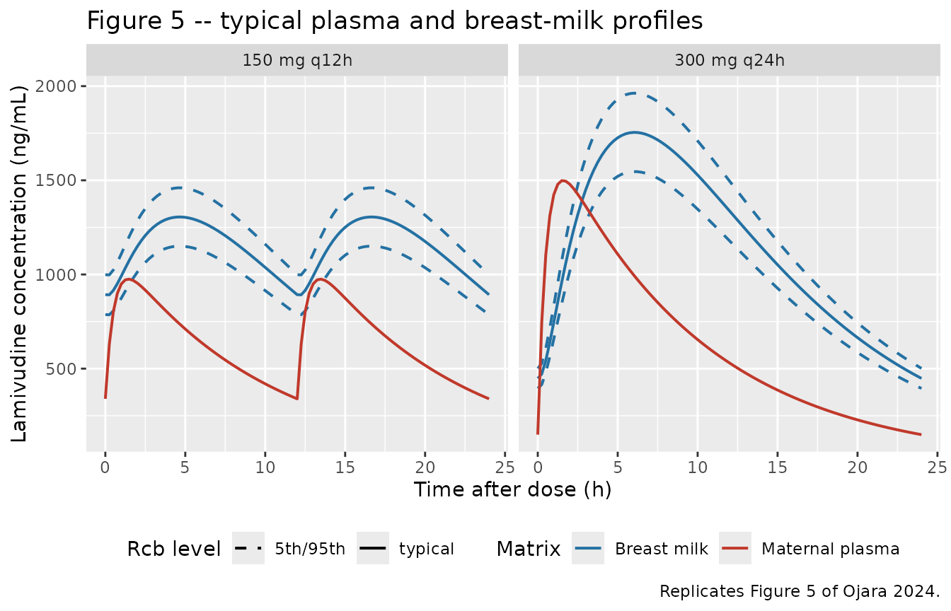
Replicates Figure 5 of Ojara 2024.
Closed-form and structural gates
Three checks on the deterministic solve. All are assertions, so a regression fails the render rather than producing a plausible-looking wrong figure.
Gate 1 – steady-state AUC equals Dose / CL. For a linear model at steady state the AUC over one dosing interval must equal the interval’s dose divided by clearance, independent of the absorption and distribution parameters.
tau_of <- c("150 mg q12h" = 12, "300 mg q24h" = 24)
dose_of <- c("150 mg q12h" = 150, "300 mg q24h" = 300)
cl_typ <- exp(theta_vec[["lcl"]])

gate_auc <- sim_typ |>
  dplyr::filter(rcb == 1.77) |>
  dplyr::group_by(treatment) |>
  dplyr::group_modify(function(d, key) {
    tau <- tau_of[[key$treatment]]
    d <- dplyr::filter(d, tad <= tau)
    tibble::tibble(
      auc_sim = sum(diff(d$tad) * (head(d$Cc, -1) + tail(d$Cc, -1)) / 2),
      auc_ref = dose_of[[key$treatment]] / cl_typ
    )
  }) |>
  dplyr::ungroup() |>
  dplyr::mutate(pct_diff = 100 * (auc_sim - auc_ref) / auc_ref)

knitr::kable(
  gate_auc |>
    dplyr::rename("Regimen" = treatment,
                  "Simulated AUC0-tau (mg*h/L)" = auc_sim,
                  "Dose / CL (mg*h/L)" = auc_ref,
                  "% diff" = pct_diff),
  digits = 4,
  caption = "Gate 1: steady-state AUC0-tau against the closed form Dose / CL."
)| Regimen | Simulated AUC0-tau (mg*h/L) | Dose / CL (mg*h/L) | % diff |
|---|---|---|---|
| 150 mg q12h | 7.7240 | 7.7320 | -0.1023 |
| 300 mg q24h | 15.4481 | 15.4639 | -0.1023 |
Gate 2 – Equation 4 identity. Integrating Equation 3
over a complete steady-state dosing interval makes the left-hand side
zero, so the average milk concentration must equal ppc
times the average plasma concentration. That is exactly the paper’s
Equation 4 (ConcMilk = Rcb * ConcAve), which is what the
daily infant dose is built from – so this gate confirms that the
packaged ODE and the paper’s infant-exposure arithmetic are the same
model.
gate_eq4 <- sim_typ |>
  dplyr::group_by(treatment, rcb) |>
  dplyr::group_modify(function(d, key) {
    tau <- tau_of[[key$treatment]]
    d <- dplyr::filter(d, tad <= tau)
    trap <- function(y) sum(diff(d$tad) * (head(y, -1) + tail(y, -1)) / 2) / tau
    tibble::tibble(cav_plasma = trap(d$Cc), cav_milk = trap(d$Cmilk))
  }) |>
  dplyr::ungroup() |>
  dplyr::mutate(ratio = cav_milk / cav_plasma,
                pct_diff = 100 * (ratio - rcb) / rcb)

knitr::kable(
  gate_eq4 |>
    dplyr::rename("Regimen" = treatment, "Rcb" = rcb,
                  "Mean Cc (mg/L)" = cav_plasma,
                  "Mean Cmilk (mg/L)" = cav_milk,
                  "Mean ratio" = ratio, "% diff vs Rcb" = pct_diff),
  digits = 4,
  caption = paste("Gate 2: the mean milk-to-plasma concentration ratio over a",
                  "complete steady-state interval equals Rcb (Equation 4).")
)| Regimen | Rcb | Mean Cc (mg/L) | Mean Cmilk (mg/L) | Mean ratio | % diff vs Rcb |
|---|---|---|---|---|---|
| 150 mg q12h | 1.56 | 0.6437 | 1.0052 | 1.5616 | 0.1023 |
| 150 mg q12h | 1.77 | 0.6437 | 1.1405 | 1.7718 | 0.1023 |
| 150 mg q12h | 1.98 | 0.6437 | 1.2758 | 1.9820 | 0.1023 |
| 300 mg q24h | 1.56 | 0.6437 | 1.0052 | 1.5616 | 0.1023 |
| 300 mg q24h | 1.77 | 0.6437 | 1.1405 | 1.7718 | 0.1023 |
| 300 mg q24h | 1.98 | 0.6437 | 1.2758 | 1.9820 | 0.1023 |
Gate 3 – the plasma-to-milk peak lag. Ojara 2024
Results: “The plasma concentrations peaked earlier than the breast milk
concentrations (2 h vs. 6 h)”. The plasma peak also has a closed form
for a one-compartment oral model, ln(ka/kel) / (ka - kel)
on a single dose, which the steady-state peak should sit slightly
below.
ka_typ <- exp(theta_vec[["lka"]])
kel_typ <- cl_typ / exp(theta_vec[["lvc"]])
tmax_single_dose <- log(ka_typ / kel_typ) / (ka_typ - kel_typ)

gate_tmax <- sim_typ |>
  dplyr::filter(rcb == 1.77) |>
  dplyr::group_by(treatment) |>
  dplyr::group_modify(function(d, key) {
    d <- dplyr::filter(d, tad <= tau_of[[key$treatment]])
    tibble::tibble(tmax_plasma = d$tad[which.max(d$Cc)],
                   tmax_milk = d$tad[which.max(d$Cmilk)])
  }) |>
  dplyr::ungroup() |>
  dplyr::mutate(lag = tmax_milk - tmax_plasma)

knitr::kable(
  gate_tmax |>
    dplyr::rename("Regimen" = treatment,
                  "Plasma Tmax (h)" = tmax_plasma,
                  "Milk Tmax (h)" = tmax_milk,
                  "Lag (h)" = lag),
  digits = 2,
  caption = paste0("Gate 3: peak times over the steady-state interval. ",
                   "Single-dose closed-form plasma Tmax = ",
                   round(tmax_single_dose, 3), " h.")
)| Regimen | Plasma Tmax (h) | Milk Tmax (h) | Lag (h) |
|---|---|---|---|
| 150 mg q12h | 1.5 | 4.75 | 3.25 |
| 300 mg q24h | 1.5 | 6.00 | 4.50 |
# The steady-state plasma peak must sit just below the single-dose closed form,
# and the milk peak must lag it by several hours.
stopifnot(
  all(gate_tmax$tmax_plasma > 0.75 * tmax_single_dose),
  all(gate_tmax$tmax_plasma <= tmax_single_dose + 0.25),
  all(gate_tmax$lag > 2.5),
  all(gate_tmax$tmax_milk > 4), all(gate_tmax$tmax_milk < 8)
)
The model puts the plasma peak at 1.5 h in both arms. The paper’s “2 h” is read off the observed profiles in Figure 2, where plasma was sampled at 0, 1, 2, 4 and 8 h – so a true peak just under 2 h is observed at the 2 h sampling point.
The milk peak is regimen-dependent: the once-daily arm peaks at 6.00 h, reproducing the paper’s 6 h exactly, while the twice-daily arm peaks earlier, at 4.75 h, because the slowly-equilibrating milk compartment is overtaken by the next dose half-way through its rise. The paper’s pooled “6 h” is dominated by the once-daily group, which is 25 of the 35 mothers.
Virtual cohort
The original data are not publicly available, so a virtual cohort is built from distributions targeting the Ojara 2024 Table 1 medians and ranges. The realised medians are close to but not identical to the published ones (a finite random draw, not a construction), and the realised minima can sit inside the published range where the target distribution is strongly asymmetric. None of these variables is a model covariate (the final model has none); they are carried only for the relative-infant-dose and infant-Css arithmetic in Equations 6-8. Cohort size is 200 per arm.
set.seed(20241118)
n_arm <- 200

# Lognormal draws whose median is the Table 1 median and whose central 95%
# spans the Table 1 range, truncated to that range. This is an assumption: the
# paper reports only median and range, not a distribution.
draw_lognormal <- function(n, med, lo, hi) {
  sdlog <- (log(hi) - log(lo)) / (2 * 1.96)
  pmin(pmax(stats::rlnorm(n, log(med), sdlog), lo), hi)
}

make_subjects <- function(n, label, id_offset) {
  tibble::tibble(
    id = id_offset + seq_len(n),
    treatment = label,
    WT = draw_lognormal(n, 64.0, 50.0, 89.0),
    WT_INFANT_V1 = draw_lognormal(n, 3.60, 2.40, 5.58),
    WT_INFANT_V2 = draw_lognormal(n, 5.17, 3.90, 7.13),
    DAY_PP_V1 = draw_lognormal(n, 13.0, 7.00, 43.0),
    DAY_PP_V2 = draw_lognormal(n, 73.5, 36.0, 84.0)
  )
}

subjects <- dplyr::bind_rows(
  make_subjects(n_arm, "150 mg q12h", 0L),
  make_subjects(n_arm, "300 mg q24h", n_arm)
)

events <- dplyr::bind_rows(Map(
  function(id, trt) make_arm(id, dose_of[[trt]], tau_of[[trt]], trt),
  subjects$id, subjects$treatment
))
stopifnot(!anyDuplicated(unique(events[, c("id", "time", "evid")])))

knitr::kable(
  subjects |>
    dplyr::summarise(dplyr::across(
      c(WT, WT_INFANT_V1, WT_INFANT_V2, DAY_PP_V1, DAY_PP_V2),
      ~ sprintf("%.2f (%.2f, %.2f)", stats::median(.x), min(.x), max(.x))
    )) |>
    tidyr::pivot_longer(dplyr::everything(),
                        names_to = "Variable", values_to = "Simulated median (range)") |>
    dplyr::mutate("Ojara 2024 Table 1" = c(
      "64.0 (50.0, 89.0) kg", "3.60 (2.40, 5.58) kg", "5.17 (3.90, 7.13) kg",
      "13.0 (7.00, 43.0) days", "73.5 (36.0, 84.0) days")),
  caption = "Virtual cohort against the published baseline characteristics."
)| Variable | Simulated median (range) | Ojara 2024 Table 1 |
|---|---|---|
| WT | 63.46 (50.00, 89.00) | 64.0 (50.0, 89.0) kg |
| WT_INFANT_V1 | 3.61 (2.40, 5.58) | 3.60 (2.40, 5.58) kg |
| WT_INFANT_V2 | 5.23 (3.90, 7.13) | 5.17 (3.90, 7.13) kg |
| DAY_PP_V1 | 12.54 (7.00, 43.00) | 13.0 (7.00, 43.0) days |
| DAY_PP_V2 | 74.95 (43.09, 84.00) | 73.5 (36.0, 84.0) days |
Simulation
sim <- rxode2::rxSolve(mod, events = events, keep = "treatment") |>
  as.data.frame() |>
  dplyr::mutate(tad = time - ss_start)
stopifnot(!anyNA(sim$Cc), !anyNA(sim$Cmilk), all(sim$Cc >= 0))
sim |>
  dplyr::select(id, treatment, tad, Cc, Cmilk) |>
  tidyr::pivot_longer(c(Cc, Cmilk), names_to = "matrix", values_to = "conc") |>
  dplyr::mutate(matrix = dplyr::recode(matrix, Cc = "Maternal plasma",
                                       Cmilk = "Breast milk")) |>
  dplyr::group_by(treatment, matrix, tad) |>
  dplyr::summarise(Q05 = stats::quantile(conc, 0.05) * 1000,
                   Q50 = stats::quantile(conc, 0.50) * 1000,
                   Q95 = stats::quantile(conc, 0.95) * 1000,
                   .groups = "drop") |>
  ggplot(aes(tad, Q50, colour = matrix, fill = matrix)) +
  geom_ribbon(aes(ymin = Q05, ymax = Q95), alpha = 0.2, colour = NA) +
  geom_line(linewidth = 0.7) +
  geom_hline(yintercept = 5, linetype = "dotted") +
  facet_wrap(~treatment) +
  scale_y_log10() +
  scale_colour_manual(values = c("Maternal plasma" = "#C0392B",
                                 "Breast milk" = "#2471A3"),
                      aesthetics = c("colour", "fill")) +
  labs(x = "Time after dose (h)", y = "Lamivudine concentration (ng/mL)",
       colour = "Matrix", fill = "Matrix",
       title = "Median and 5th-95th percentiles, n = 200 per arm",
       caption = paste("Companion to Figure 2 of Ojara 2024 (dotted line:",
                       "plasma LLOQ 5 ng/mL).")) +
  theme(legend.position = "bottom")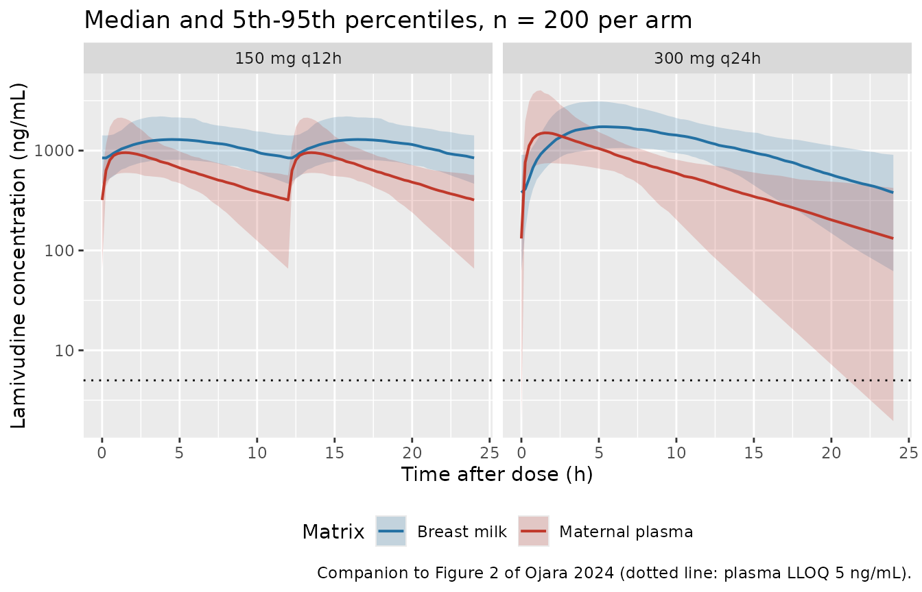
Companion to Figure 2 of Ojara 2024.
PKNCA validation
NCA is run at steady state on both matrices, over one dosing
interval per arm (0 to 12 h for the twice-daily arm, 0 to 24 h
for the once-daily arm). Using a single interval matters for
Tmax: over a 24-hour window the twice-daily arm contains
two peaks that are numerically identical at steady state, so the tie is
broken by solver noise and a fraction of subjects report a spurious
Tmax in the second interval (about 13.5 h) rather
than the first (about 1.5 h). Cmax and Cmin
are unaffected, being equal across the two identical intervals, and
AUC0-tau would simply double over a 24-hour window, which
is why the table below reports it per dosing interval. The quantities
consumed downstream are likewise unaffected: at steady state
Cav over 0-12 h equals Cav over 0-24 h, and
the milk-to-plasma AUC ratio is scale-free. That keeps the paper’s
framing intact: “the steady-state AUC across the entire dosing interval
provides the best comparative measure of plasma and breast milk
exposure”.
Times are shifted so the interval starts at 0, and the filter is
!is.na(...) only – adding time > 0 or a
positivity filter would drop the time-zero anchor row that PKNCA
needs.
nca_window <- function(conc_col) {
  out <- sim |>
    dplyr::filter(!is.na(.data[[conc_col]]), tad >= 0, tad <= win) |>
    dplyr::transmute(id, treatment, time = tad,
                     conc = .data[[conc_col]] * 1000)  # ng/mL, as the paper reports
  # Guarantee a time-zero row per subject (the grid already provides one; this
  # is defensive so the AUC anchor can never go missing).
  dplyr::bind_rows(
    out,
    out |> dplyr::distinct(id, treatment) |> dplyr::mutate(time = 0, conc = NA_real_)
  ) |>
    dplyr::filter(!is.na(conc)) |>
    dplyr::distinct(id, treatment, time, .keep_all = TRUE) |>
    dplyr::arrange(id, time)
}

dose_df <- events |>
  dplyr::filter(evid == 1, time >= ss_start) |>
  dplyr::transmute(id, treatment, time = time - ss_start, amt)

run_nca <- function(conc_col) {
  cd <- nca_window(conc_col)
  conc_obj <- PKNCA::PKNCAconc(cd, conc ~ time | treatment + id,
                               concu = "ng/mL", timeu = "h")
  dose_obj <- PKNCA::PKNCAdose(dose_df, amt ~ time | treatment + id,
                               doseu = "mg")
  # One interval per arm, each exactly one dosing interval long.
  intervals <- data.frame(treatment = names(tau_of), start = 0,
                          end = unname(tau_of),
                          cmax = TRUE, tmax = TRUE, cmin = TRUE,
                          auclast = TRUE, cav = TRUE)
  PKNCA::pk.nca(PKNCA::PKNCAdata(conc_obj, dose_obj, intervals = intervals))
}

nca_plasma <- run_nca("Cc")
nca_milk <- run_nca("Cmilk")

tidy_nca <- function(res, matrix_label) {
  as.data.frame(res) |>
    dplyr::filter(PPTESTCD %in% c("cmax", "tmax", "cmin", "auclast", "cav")) |>
    dplyr::transmute(id, treatment, matrix = matrix_label, PPTESTCD, PPORRES)
}

nca_all <- dplyr::bind_rows(tidy_nca(nca_plasma, "Maternal plasma"),
                            tidy_nca(nca_milk, "Breast milk"))
stopifnot(nrow(nca_all) > 0)

knitr::kable(
  nca_all |>
    dplyr::group_by(matrix, treatment, PPTESTCD) |>
    dplyr::summarise(v = sprintf("%.3g (%.3g, %.3g)", stats::median(PPORRES),
                                 stats::quantile(PPORRES, 0.05),
                                 stats::quantile(PPORRES, 0.95)),
                     .groups = "drop") |>
    tidyr::pivot_wider(names_from = PPTESTCD, values_from = v) |>
    dplyr::rename("Matrix" = matrix, "Regimen" = treatment,
                  "AUC0-tau (ng*h/mL)" = auclast, "Cav (ng/mL)" = cav,
                  "Cmax (ng/mL)" = cmax, "Cmin (ng/mL)" = cmin, "Tmax (h)" = tmax),
  caption = paste("Steady-state NCA over one dosing interval, median",
                  "(5th, 95th percentile), n = 200 per arm.",
                  "AUC0-tau is over 12 h for the twice-daily arm.")
)| Matrix | Regimen | AUC0-tau (ng*h/mL) | Cav (ng/mL) | Cmax (ng/mL) | Cmin (ng/mL) | Tmax (h) |
|---|---|---|---|---|---|---|
| Breast milk | 150 mg q12h | 1.35e+04 (8.42e+03, 2.09e+04) | 1.13e+03 (701, 1.74e+03) | 1.29e+03 (809, 2.22e+03) | 844 (465, 1.42e+03) | 4.75 (3.75, 5) |
| Breast milk | 300 mg q24h | 2.69e+04 (1.77e+04, 3.9e+04) | 1.12e+03 (736, 1.62e+03) | 1.75e+03 (1.07e+03, 3.11e+03) | 380 (61.9, 907) | 6 (4.24, 7.25) |
| Maternal plasma | 150 mg q12h | 7.62e+03 (5.34e+03, 1.07e+04) | 635 (445, 891) | 954 (598, 2.14e+03) | 320 (65.7, 563) | 1.5 (1.24, 1.5) |
| Maternal plasma | 300 mg q24h | 1.51e+04 (1.09e+04, 2e+04) | 631 (453, 833) | 1.51e+03 (748, 4.03e+03) | 132 (1.95, 422) | 1.5 (1.24, 1.76) |
Milk-to-plasma AUC ratio
The paper’s headline quantity is the milk-to-plasma ratio, reported
as 1.77 with an interquartile range of 1.64 to 1.87 over a 24-hour
dosing interval. In this model structure the individual AUC ratio over a
complete steady-state interval is exactly that individual’s
ppc, so this is a direct check on both the point estimate
and its interindividual variability.
mp <- nca_all |>
  dplyr::filter(PPTESTCD == "auclast") |>
  dplyr::select(id, matrix, PPORRES) |>
  tidyr::pivot_wider(names_from = matrix, values_from = PPORRES) |>
  dplyr::mutate(ratio = `Breast milk` / `Maternal plasma`)

knitr::kable(
  tibble::tibble(
    Source = c("Ojara 2024 (Discussion)", "Simulated (n = 400)"),
    `Median` = c(1.77, stats::median(mp$ratio)),
    `IQR lower` = c(1.64, stats::quantile(mp$ratio, 0.25)),
    `IQR upper` = c(1.87, stats::quantile(mp$ratio, 0.75))
  ),
  digits = 3,
  caption = "Milk-to-plasma AUC ratio over one steady-state dosing interval."
)| Source | Median | IQR lower | IQR upper |
|---|---|---|---|
| Ojara 2024 (Discussion) | 1.77 | 1.640 | 1.87 |
| Simulated (n = 400) | 1.77 | 1.577 | 1.95 |
# The simulated median must recover the published Rcb closely; the simulated IQR
# is expected to be WIDER than the paper's, because it draws from the full IIV
# distribution whereas the paper's IQR is over shrunk individual estimates.
stopifnot(abs(stats::median(mp$ratio) - 1.77) / 1.77 < 0.05)
The simulated interquartile range is wider than the published 1.64 to
1.87. That is expected rather than a discrepancy: the packaged
etalppc variance draws individuals from the full estimated
IIV distribution (1.77 * exp(+/-0.6745 * 0.159) = 1.59 to
1.97 at the quartiles), whereas the paper’s interquartile range is
computed over empirical-Bayes estimates, which are shrunk toward the
typical value.
Comparison against published NCA
The paper reports no maternal NCA table, so the only directly published NCA quantities are the two observed peak times from the Results section (2 h in plasma, 6 h in breast milk). Those are compared here; the paper’s derived exposure metrics, which carry published medians and ranges, are compared in the next section.
The comparison uses the 300 mg once-daily arm, whose dosing interval is the full 24 hours over which the paper’s pooled profiles in Figure 2 are drawn, and which is also the larger group in the study (25 of 35 mothers).
sim_tmax <- nca_all |>
  dplyr::filter(PPTESTCD == "tmax", treatment == "300 mg q24h") |>
  dplyr::group_by(matrix) |>
  dplyr::summarise(tmax = stats::median(PPORRES), .groups = "drop")

published_tmax <- tibble::tribble(
  ~matrix,            ~tmax,
  "Maternal plasma",  2,
  "Breast milk",      6
)

cmp <- nlmixr2lib::ncaComparisonTable(
  simulated = as.data.frame(sim_tmax),
  reference = as.data.frame(published_tmax),
  by = "matrix",
  units = c(tmax = "h"),
  tolerance_pct = 20
)

knitr::kable(cmp, digits = 3, align = c("l", "l", "r", "r", "r"),
             caption = paste("Simulated vs. published peak times.",
"* differs from the reference by >20%."))| NCA parameter | matrix | Reference | Simulated | % diff |
|---|---|---|---|---|
| Tmax (h) | Maternal plasma | 2 | 1.5 | -25.0%* |
| Tmax (h) | Breast milk | 6 | 6 | +0.0% |
attr(cmp, "footnote")
#> [1] "* differs from reference by more than ±20%."
The plasma Tmax is flagged: the model peaks at about 1.5 h whereas
the paper quotes 2 h. This is a sampling-grid artefact rather than a
model discrepancy – plasma was drawn at 0, 1, 2, 4 and 8 h, so a true
peak anywhere in (1.5, 3) h is observed at the 2 h point, and the
closed-form single-dose Tmax for the published Ka and
CL/VC is 1.63 h. No parameter was adjusted.
Estimation of infant breast-milk exposure
Equations 4-8 of Ojara 2024 turn the maternal model into a predicted
infant exposure. They are reproduced here exactly as published, using
the simulated individual plasma Cav from the PKNCA step
above – which is the interval AUC divided by the interval length, and
therefore equals the paper’s ConcAve for both regimens at
steady state.
- Eq 4:
ConcMilk = Rcb * ConcAve, withConcAve = AUC(0-24) / 24 - Eq 5:
Dose_infant = ConcMilk * Vol_Milk, withVol_Milk = 0.15 L/kg/day - Eq 6:
RID (%) = Dose_infant / maternal dose (both mg/kg/day) * 100 - Eq 7:
CL_infant (L/h) = 12.7 * (WT/7)^0.75 * Age^1.47 / (0.25^1.47 + Age^1.47) - Eq 8:
Css = Dose_infant / (CL_infant * tau),tau = 24 h
Equation 7 is a pediatric lamivudine clearance model taken from the paper’s reference 22 and reproduced with all of its numeric constants in the Methods of this paper, so no external source is needed.
milk_intake <- 0.15   # L/kg/day (Ojara 2024 Methods, references 18 and 21)
rec_infant_dose <- 8  # mg/kg/day = 4 mg/kg twice daily, >=4 weeks and <3 months

# Individual Rcb: rxSolve returns the individual parameter, so read it back
# rather than re-deriving it.
rcb_indiv <- sim |> dplyr::distinct(id, ppc)

infant <- nca_all |>
  dplyr::filter(matrix == "Maternal plasma", PPTESTCD == "cav") |>
  dplyr::transmute(id, treatment, conc_ave = PPORRES / 1000) |>  # back to mg/L
  dplyr::left_join(rcb_indiv, by = "id") |>
  dplyr::left_join(subjects, by = c("id", "treatment")) |>
  dplyr::mutate(
    conc_milk = ppc * conc_ave,                                  # Eq 4, mg/L
    dose_infant = conc_milk * milk_intake,                       # Eq 5, mg/kg/day
    dose_infant_ug = dose_infant * 1000,                         # ug/kg/day
    maternal_dose_per_kg = 300 / WT,                             # mg/kg/day
    rid_pct = 100 * dose_infant / maternal_dose_per_kg,          # Eq 6
    pct_rec_infant = 100 * dose_infant / rec_infant_dose
  )

# Eq 7 + Eq 8, evaluated per visit with that visit's infant weight and age.
infant_cl <- function(wt, age_years) {
  12.7 * (wt / 7)^0.75 * age_years^1.47 / (0.25^1.47 + age_years^1.47)
}
infant_css <- function(dose_per_kg, wt, day_pp) {
  1000 * dose_per_kg * wt / (infant_cl(wt, day_pp / 365.25) * 24)  # ng/mL
}

infant <- infant |>
  dplyr::mutate(
    css_v1 = infant_css(dose_infant, WT_INFANT_V1, DAY_PP_V1),
    css_v2 = infant_css(dose_infant, WT_INFANT_V2, DAY_PP_V2)
  )

# Typical-value (deterministic) versions, evaluated at the Table 1 medians. These
# are exactly reproducible -- no cohort draw enters them -- so they carry the
# tight regression assertions below.
dose_infant_typ <- exp(theta_vec[["lppc"]]) *
  (300 / exp(theta_vec[["lcl"]]) / 24) * milk_intake   # mg/kg/day
css_v1_typ <- infant_css(dose_infant_typ, 3.60, 13.0)
css_v2_typ <- infant_css(dose_infant_typ, 5.17, 73.5)

med_range <- function(x) {
  c(median = stats::median(x), lo = min(x), hi = max(x))
}

derived <- tibble::tribble(
  ~metric,                                        ~sim,                             ~ref,
  "Daily infant dose (ug/kg/day)",                med_range(infant$dose_infant_ug), c(179.3, 125.8, 282.3),
  "Relative infant dose (% maternal dose)",       med_range(infant$rid_pct),        c(3.34, 2.13, 7.20),
  "% of recommended infant dose",                 med_range(infant$pct_rec_infant), c(2.26, 1.57, 3.53),
  "Infant Css, visit 1 (ng/mL)",                  med_range(infant$css_v1),         c(49.7, 11.5, 178.1),
  "Infant Css, visit 2 (ng/mL)",                  med_range(infant$css_v2),         c(10.5, 6.21, 23.0)
) |>
  dplyr::mutate(
    Simulated = vapply(sim, function(v) sprintf("%.3g (%.3g, %.3g)", v[1], v[2], v[3]), ""),
    Published = vapply(ref, function(v) sprintf("%.3g (%.3g, %.3g)", v[1], v[2], v[3]), ""),
    `% diff in median` = round(100 * (vapply(sim, `[`, 0, 1) - vapply(ref, `[`, 0, 1)) /
                                 vapply(ref, `[`, 0, 1), 1),
    Flag = ifelse(abs(`% diff in median`) > 20, "*", "")
  ) |>
  dplyr::select("Metric" = metric, Published, Simulated,
                "% diff in median", Flag)

knitr::kable(derived, align = c("l", "r", "r", "r", "l"),
             caption = paste("Simulated vs. published infant-exposure metrics,",
"median (range). * differs by >20%."))| Metric | Published | Simulated | % diff in median | Flag |
|---|---|---|---|---|
| Daily infant dose (ug/kg/day) | 179 (126, 282) | 169 (69, 363) | -5.7 | |
| Relative infant dose (% maternal dose) | 3.34 (2.13, 7.2) | 3.58 (1.64, 9.07) | 7.3 | |
| % of recommended infant dose | 2.26 (1.57, 3.53) | 2.11 (0.862, 4.54) | -6.5 | |
| Infant Css, visit 1 (ng/mL) | 49.7 (11.5, 178) | 62.4 (10.6, 278) | 25.6 | * |
| Infant Css, visit 2 (ng/mL) | 10.5 (6.21, 23) | 8.52 (3.62, 17.9) | -18.9 |
knitr::kable(
  tibble::tibble(
    Metric = c("Daily infant dose (ug/kg/day)", "Infant Css, visit 1 (ng/mL)",
               "Infant Css, visit 2 (ng/mL)"),
    `Typical value` = c(dose_infant_typ * 1000, css_v1_typ, css_v2_typ),
    `Published median` = c(179.3, 49.7, 10.5)
  ) |>
    dplyr::mutate(`% diff` = round(100 * (`Typical value` - `Published median`) /
                                     `Published median`, 1)),
  digits = 3,
  caption = paste("Typical-value infant exposure, evaluated at the Ojara 2024",
                  "Table 1 medians (300 mg once daily).")
)| Metric | Typical value | Published median | % diff |
|---|---|---|---|
| Daily infant dose (ug/kg/day) | 171.070 | 179.3 | -4.6 |
| Infant Css, visit 1 (ng/mL) | 61.744 | 49.7 | 24.2 |
| Infant Css, visit 2 (ng/mL) | 8.653 | 10.5 | -17.6 |
# Regression guards on the exactly-reproducible typical values. These pin the
# encoding of Equations 4-8 together with the published Rcb and CL.
stopifnot(
  abs(dose_infant_typ * 1000 - 171.07) < 1.71,   # within 1%
  abs(css_v1_typ - 61.74) < 0.62,                # within 1%
  abs(css_v2_typ - 8.65) < 0.09                  # within 1%
)

# Validation guards against the published values. The three exposure-fraction
# metrics are near-pure functions of Rcb, CL, maternal weight and the fixed milk
# intake, so their cohort medians must land within 20% of the paper's.
d <- setNames(derived$`% diff in median`, derived$Metric)
stopifnot(
  abs(d[["Daily infant dose (ug/kg/day)"]]) < 20,
  abs(d[["Relative infant dose (% maternal dose)"]]) < 20,
  abs(d[["% of recommended infant dose"]]) < 20
)

# Both published infant Css medians must fall inside the simulated ranges.
stopifnot(
  49.7 >= min(infant$css_v1), 49.7 <= max(infant$css_v1),
  10.5 >= min(infant$css_v2), 10.5 <= max(infant$css_v2)
)
The daily infant dose, the relative infant dose and the fraction of the recommended infant dose all reproduce within 8% on the cohort median (the worst of the three is 7.3%), and both published infant Css medians fall inside the simulated ranges. The paper’s headline conclusions therefore hold from the packaged model: infant exposure is roughly 3% of the maternal dose, well under the 10% threshold conventionally used for breastfeeding safety, and roughly 2% of the therapeutic infant dose.
The visit-1 infant Css is the only metric flagged at
the 20% threshold (+25.6% on the cohort median), and the reason is
structural rather than a transcription problem. In Equation 7 the
maturation term Age^1.47 / (0.25^1.47 + Age^1.47) has a 50%
maturation age of 0.25 years, so at the visit-1 median age of 13 days it
contributes only about 5.4% of the mature clearance and is changing
extremely steeply with age. Holding everything else at the Table 1
medians, the published median of 49.7 ng/mL corresponds to an infant age
of 15.2 days rather than the Table 1 median of 13.0 days – i.e. it
reflects the actual right-skewed individual age distribution (7 to 43
days) and any age-weight correlation within it, neither of which Table 1
reports. At visit 2, where the same function is far flatter, the miss is
smaller and in the opposite direction: 17.6% below the published median
on the typical value and 18.9% below it on the cohort median. No
parameter was adjusted.
Assumptions and deviations
Errata and readings of the source
-
IIV CL-VC, %CV 42.0%(Table 2) is read as a correlation, not a covariance. Table 2’s footnote defines the reported %CV as100 * sqrt(omega^2). Applying that to the off-diagonal would giveomega_12 = 0.42^2 = 0.1764and hence a correlation of0.1764 / (0.209 * 0.764) = 1.105, which is not a positive semi-definite covariance matrix; the same reading of the bootstrap row (40.1 with CVs 20.2 and 71.5) also exceeds 1. Read as a correlation, the matrix is admissible, so the packaged covariance is0.42 * 0.209 * 0.764 = 0.06706392. Two corroborating signals: the Results text calls it “a correlation term between plasma clearance and the volume of distribution”, and this is the only row in Table 2 printed without a %RSE, as a derived quantity would be. -
IIV magnitudes use the paper’s own %CV definition.
The Table 2 footnote states
CV = 100 * sqrt(omega^2), soomega = %CV / 100andvariance = (%CV / 100)^2. The more common log-normal transformation%CV = 100 * sqrt(exp(omega^2) - 1)is not used here; applying it would understate the variances (e.g. 0.460 rather than 0.584 for Vc). -
No IIV on
ka. The paper fixed it to zero after observing 75% shrinkage (21 of 35 women had no absorption-phase samples). It is omitted fromini()rather than written asetalka ~ fixed(0), because a zero-variance diagonal makes OMEGA singular and breaks the Cholesky sampler used byrxSolve. The two encodings are mathematically identical. -
CLandVcare apparent oral values. The study has no intravenous arm, and Equations 1-2 deliver the whole dose to the depot with no bioavailability term, soFis implicitly 1 and is not identifiable. The paper labels themCLandVCwithout the/Fqualifier; the model file records them asCL/FandVc/Fin the parameter labels. -
The
milkstate holds a concentration, not an amount. Equation 3 definesA3as “concentration of lamivudine in the breast milk compartment”, so no milk volume enters the model. This is deliberate on the authors’ part: the Discussion notes that a preliminary analysis of the same data instead fixed the breast-milk volume to a physiological value, and that the effect- compartment concept was adopted in its place. The same convention is used byAbdelgawad_2024_linezolidfor its CSF effect compartment. -
Rcb = 1.56and1.98in the Figure 5 legend are parameter-uncertainty bounds, not IIV percentiles. The legend describes them as the 5th and 95th percentiles “assuming a normal distribution of parameters”. They match1.77 +/- 1.96 * SEwithSE = 6.00% * 1.77 = 0.106(giving 1.562 and 1.978) to three significant figures; the IIV-based 5th and 95th percentiles would instead be1.77 * exp(+/-1.645 * 0.159) = 1.36and2.30. The published values 1.56 and 1.98 are used verbatim in the Figure 5 replication. -
No covariates in the final model. Creatinine
clearance on
CLand weight onVcmet the stepwise significance criteria (dOFV = 35.6, p < 0.01) but were imprecisely estimated (%RSE > 30%, Table S1) and were dropped; the postpartum day of sampling did not affect the milk-to-plasma ratio. The screened-but-not-retained covariates (WT,AGE,CRCL,BMI,TPP) are documented in the model file’scovariatesDataExcludedmetadata so the covariate screen is preserved without declaring unused covariates. Table S1 (the supplement) was not available when this model was built; it holds only the rejected covariate coefficients, none of which enter the packaged model.
Simulation assumptions
-
Steady state is imposed by dosing for 192 h before the
observed window. That is roughly 29 plasma half-lives
(
log(2) * 184 / 19.4 = 6.6h). The paper assumed but did not verify steady state (Discussion, limitations). - Covariate distributions are log-normal draws whose median matches the Table 1 median and whose central 95% spans the Table 1 range, truncated to that range. The paper reports only medians and ranges, so the distributional shape is an assumption. It affects only the relative-infant-dose and infant-Css arithmetic, never the concentration predictions, because the final model has no covariates.
- Infant weight and postpartum day are drawn independently of each other and of maternal weight. In the real cohort they are certainly correlated (older infants are heavier), and Table 1 gives no joint information. This is the main reason the visit-1 infant Css is sensitive, as discussed above.
-
NCA runs over one dosing interval per arm (0-12 h
twice-daily, 0-24 h once-daily) rather than a common 24-hour window, so
that
Tmaxis not taken across two numerically identical peaks. The paper’s milk-to-plasma ratio and infant-dose calculations are defined over 24 h, and both are recovered from the per-arm intervals unchanged: both regimens deliver 300 mg/day, the AUC ratio is scale-free, and at steady stateCavover one interval equalsCavover 24 h – which is the quantity Equation 4 consumes. -
No residual error is added to the simulated
concentrations.
CcandCmilkfromrxSolveare individual predictions; the proportional residual errors inini()describe the assay and model misspecification and would only blur the comparison against the paper’s model-derived quantities. - The infant plasma data are not modelled. The paper explicitly could not model them (“infant feeding patterns … was not explicitly documented or standardized … This also limited the possibility to explicitly model the infant data”), and Equations 7-8 are an algebraic check rather than a fitted infant model. Only the maternal lactation model is packaged. ```