Model and source
- Citation: Ma K-f, Liu Y-x, Jiao Z, Lv J-h, Yang P, Wu J-y, Yang S. Population Pharmacokinetics of Vancomycin in Kidney Transplant Recipients: Model Building and Parameter Optimization. Front Pharmacol. 2020;11:563967. doi:10.3389/fphar.2020.563967
- Description: One-compartment IV population PK model for vancomycin in 56 adult Chinese kidney transplant recipients receiving prophylactic vancomycin in the first postoperative weeks (Ma 2020). Clearance scales by power functions of body weight (reference 59.95 kg) and raw estimated glomerular filtration rate (mL/min, reference 36.67); volume of distribution scales by a power function of body weight. IIV on CL only; proportional residual error. Estimated from 195 trough concentrations collected by routine therapeutic drug monitoring.
- Article: https://doi.org/10.3389/fphar.2020.563967 (open access, CC BY 4.0)
Population
Ma 2020 is a retrospective, single-centre therapeutic-drug-monitoring (TDM) study at the First Affiliated Hospital of Zhejiang University School of Medicine, Hangzhou. Fifty-six adult kidney transplant recipients (35 male, 21 female; all grafts from brain-dead donors) received intravenous vancomycin as postoperative prophylaxis after surgery between March and June 2017 (Methods, “Patients and Data Collection”). Table 1 reports age 43.72 +/- 9.92 years (range 24-70), body weight 58.27 +/- 8.47 kg (median 59.95, range 37.7-79), serum creatinine median 164 umol/L (range 60-1,490) and estimated GFR median 39.91 mL/min (IQR 32.53-59.44, range 3.38-108.61). Nearly all patients received prednisone, mycophenolate mofetil and tacrolimus (four received cyclosporine A instead).
Vancomycin was given as 500 mg per administration: one dose on the first postoperative day, then 1-4 administrations per day (500-2,000 mg/day) adjusted by TDM (Methods, “Drug Administration”). All 195 concentrations are troughs drawn about 30 min before the morning dose, first sampled a median 4 days after transplantation (Table 1). The fit used NONMEM 7.4 with FOCE-I.
The same information is stored in the model’s population
metadata.
Source trace
| Model element | Value | Source location |
|---|---|---|
| Structure | one-compartment, IV input, first-order elimination | Methods, “Population Pharmacokinetic Modeling” |
lcl |
log(2.08 L/h) | Table 2 final model, CL |
lvc |
log(63.2 L) | Table 2 final model, V |
e_crcl_cl |
0.698 | Table 2, theta_1 (GFR on CL) |
e_wt_cl |
1.07 | Table 2, theta_2 (WT on CL) |
e_wt_vc |
0.934 | Table 2, theta_3 (WT on V) |
| CL equation | 2.08 * (WT/59.95)^1.07 * (GFR/36.67)^0.698 |
Results, “Assessment of Covariates and Evaluation of Models” |
| V equation | 63.2 * (WT/59.95)^0.934 |
Results, same section |
etalcl |
log(0.215^2 + 1) = 0.04517 | Table 2, omega_1 = 21.5% (CV reading; see below) |
| IIV on V | none | Table 2 prints no omega for V |
propSd |
0.242 | Table 2, sigma_1 = 24.2%; Results: proportional model selected |
| Validation target | 15 weight/GFR daily-dose regimens, each >90% AUC0-24 >= 400 | Table 3; Methods, “Model Application” |
The omega scale
Table 2 heads its IIV row “Intersubject variance of CL” and prints
21.5%. That could be a coefficient of variation (omega^2 = log(0.215^2 +
1) = 0.0452) or the variance itself (omega^2 = 0.215, a CV of about
49%). Table 3 separates the two. Its 15 daily-dose recommendations are
each reported to give more than 90% of patients an AUC0-24 of at least
400 mg*h/L (MIC 1 mg/L). At steady state AUC0-24 = daily dose / CL
exactly, and CL is log-normal, so the fraction reaching the target is
available in closed form:
P(AUC >= 400) = pnorm(log(dose / (400 * CL_typ)) / omega).
# Ma 2020 Table 3, transcribed.
table3 <- expand.grid(GFR = c(30, 45, 60, 75, 90), WT = c(40, 50, 60)) |>
  dplyr::select(WT, GFR) |>
  dplyr::mutate(
    daily_dose = c(
      750, 1000, 1250, 1500, 1750,
      1000, 1250, 1500, 1750, 2000,
      1250, 1500, 1750, 2250, 2500
    ),
    scenario = sprintf("WT %d kg, GFR %d mL/min", WT, GFR)
  )

cl_typ <- function(wt, gfr) 2.08 * (wt / 59.95)^1.07 * (gfr / 36.67)^0.698

pta_closed <- table3 |>
  dplyr::mutate(
    cl_typical = cl_typ(WT, GFR),
    pta_cv = pnorm(log(daily_dose / (400 * cl_typical)) / sqrt(log(1 + 0.215^2))),
    pta_variance = pnorm(log(daily_dose / (400 * cl_typical)) / sqrt(0.215))
  )

pta_closed |>
  dplyr::select(WT, GFR, daily_dose, cl_typical, pta_cv, pta_variance) |>
  dplyr::mutate(dplyr::across(c(pta_cv, pta_variance), ~ 100 * .x)) |>
  dplyr::rename(
    "WT (kg)" = WT,
    "GFR (mL/min)" = GFR,
    "Daily dose (mg)" = daily_dose,
    "Typical CL (L/h)" = cl_typical,
    "% AUC0-24 >= 400, CV reading" = pta_cv,
    "% AUC0-24 >= 400, variance reading" = pta_variance
  ) |>
knitr::kable(digits = c(0, 0, 0, 2, 1, 1))| WT (kg) | GFR (mL/min) | Daily dose (mg) | Typical CL (L/h) | % AUC0-24 >= 400, CV reading | % AUC0-24 >= 400, variance reading |
|---|---|---|---|---|---|
| 40 | 30 | 750 | 1.17 | 98.6 | 84.4 |
| 40 | 45 | 1000 | 1.56 | 98.7 | 84.7 |
| 40 | 60 | 1250 | 1.90 | 99.0 | 85.8 |
| 40 | 75 | 1500 | 2.22 | 99.3 | 87.0 |
| 40 | 90 | 1750 | 2.52 | 99.5 | 88.2 |
| 50 | 30 | 1000 | 1.49 | 99.3 | 86.8 |
| 50 | 45 | 1250 | 1.98 | 98.4 | 83.9 |
| 50 | 60 | 1500 | 2.42 | 98.1 | 82.9 |
| 50 | 75 | 1750 | 2.82 | 98.0 | 82.8 |
| 50 | 90 | 2000 | 3.21 | 98.2 | 83.1 |
| 60 | 30 | 1250 | 1.81 | 99.5 | 88.1 |
| 60 | 45 | 1500 | 2.40 | 98.2 | 83.2 |
| 60 | 60 | 1750 | 2.94 | 97.0 | 80.5 |
| 60 | 75 | 2250 | 3.43 | 99.0 | 85.7 |
| 60 | 90 | 2500 | 3.90 | 98.7 | 84.6 |
# Deterministic (closed form, no simulation). The CV reading reproduces the
# paper's '>90%' in every cell; the variance reading fails every cell.
stopifnot(
  all(pta_closed$pta_cv > 0.90),
  all(pta_closed$pta_variance < 0.90)
)
The CV reading gives 97-99.5% in every cell and the variance reading gives only 80-88%, so the variance reading contradicts every row of Table 3. The model uses the CV reading. The residual row (24.2%) is read on the same scale as a proportional SD of 0.242.
Virtual cohort
Each of the 15 Table 3 scenarios is simulated as its own arm of 200 subjects with weight and GFR fixed at the scenario values. The daily dose is split into two 12-hourly 1-hour infusions (the paper gives neither the split nor the infusion time; neither affects AUC0-24 at steady state) for 20 days, so the last day is at steady state for every subject (the typical half-life is 11-26 h across the scenarios, and a subject with low clearance in the lightest, lowest-GFR scenario reaches about 45 h; 10 days would leave such subjects a few percent short of steady state).
# rxSetSeed() fixes the draw within an rxode2 build; the assertions below are
# written to hold for any cohort the model can produce.
rxode2::rxSetSeed(2020)

mod <- readModelDb("Ma_2020_vancomycin")
n_per_arm <- 200L
tau <- 12
n_doses <- 40L
t_inf <- 1
t_last <- n_doses * tau

make_arm <- function(i) {
  row <- table3[i, ]
  ids <- (i - 1L) * n_per_arm + seq_len(n_per_arm)
  dose_rows <- expand.grid(id = ids, time = (seq_len(n_doses) - 1L) * tau) |>
    dplyr::mutate(evid = 1L, amt = row$daily_dose / 2, dur = t_inf)
  obs_times <- sort(unique(c(seq(0, t_last, by = 2), seq(t_last - 24, t_last, by = 0.25))))
  obs_rows <- expand.grid(id = ids, time = obs_times) |>
    dplyr::mutate(evid = 0L, amt = 0, dur = 0)
  dplyr::bind_rows(dose_rows, obs_rows) |>
    dplyr::mutate(
      cmt = "central",
      WT = row$WT,
      CRCL = row$GFR,
      scenario = row$scenario
    ) |>
    dplyr::arrange(id, time, dplyr::desc(evid))
}

events <- dplyr::bind_rows(lapply(seq_len(nrow(table3)), make_arm))
stopifnot(dplyr::n_distinct(events$id) == n_per_arm * nrow(table3))Replicate published figures
The paper’s figures are observed data and diagnostics (Figure 1, observed troughs; Figures 3-5, goodness of fit and NPDE), so no model-predicted figure is available to overlay. The figure below shows the simulated median and 90% interval of the concentration-time profile over the final (steady-state) day for the 60 kg scenarios, the heaviest weight band in Table 3.
sim |>
  dplyr::filter(WT == 60, time >= t_last - 24) |>
  dplyr::group_by(scenario, time) |>
  dplyr::summarise(
    q05 = quantile(Cc, 0.05), q50 = median(Cc), q95 = quantile(Cc, 0.95),
    .groups = "drop"
  ) |>
  ggplot(aes(time - (t_last - 24), q50, colour = scenario, fill = scenario)) +
  geom_ribbon(aes(ymin = q05, ymax = q95), alpha = 0.15, colour = NA) +
  geom_line() +
  labs(
    x = "Time within day 20 (h)", y = "Vancomycin (mg/L)",
    colour = NULL, fill = NULL,
    title = "Table 3 regimens, 60 kg: day-20 profile (median, 90% interval)"
  ) +
  theme_bw()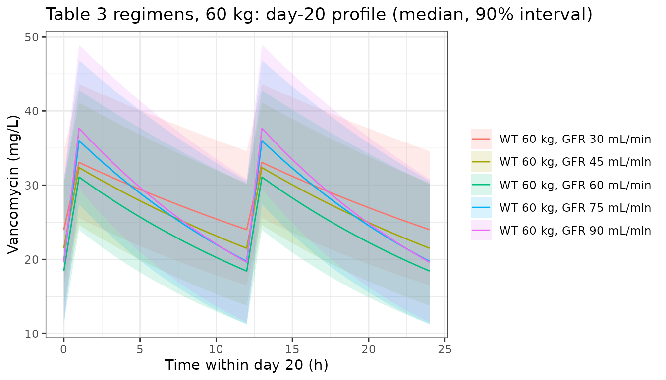
Deterministic structural checks
With random effects zeroed, the model’s clearance and volume must equal the Results equations exactly.
mod_typical <- rxode2::zeroRe(mod)
#> ℹ parameter labels from comments will be replaced by 'label()'
ev_typ <- events |>
  dplyr::filter(id %in% ((seq_len(nrow(table3)) - 1L) * n_per_arm + 1L))
sim_typ <- rxode2::rxSolve(
  mod_typical, ev_typ,
  keep = c("scenario", "WT", "CRCL"),
  returnType = "data.frame"
)
#> ℹ omega/sigma items treated as zero: 'etalcl'
#> Warning: multi-subject simulation without without 'omega'
chk_eq <- sim_typ |>
  dplyr::distinct(scenario, WT, CRCL, cl, vc) |>
  dplyr::mutate(
    cl_paper = cl_typ(WT, CRCL),
    vc_paper = 63.2 * (WT / 59.95)^0.934
  )
stopifnot(nrow(chk_eq) == nrow(table3))
stopifnot(
  max(abs(chk_eq$cl / chk_eq$cl_paper - 1)) < 1e-10,
  max(abs(chk_eq$vc / chk_eq$vc_paper - 1)) < 1e-10
)
PKNCA validation
AUC is computed with PKNCA over the final day (456-480 h) for every simulated subject, grouped by scenario.
conc_df <- sim |>
  dplyr::filter(!is.na(Cc), time >= t_last - 24) |>
  dplyr::select(id, time, Cc, scenario)

dose_df <- events |>
  dplyr::filter(evid == 1L) |>
  dplyr::select(id, time, amt, scenario)

conc_obj <- PKNCA::PKNCAconc(conc_df, Cc ~ time | scenario + id)
dose_obj <- PKNCA::PKNCAdose(dose_df, amt ~ time | scenario + id)
intervals <- data.frame(
  start = t_last - 24, end = t_last,
  auclast = TRUE, cmax = TRUE, cmin = TRUE
)
nca_res <- PKNCA::pk.nca(
  PKNCA::PKNCAdata(conc_obj, dose_obj, intervals = intervals)
)

nca_wide <- as.data.frame(nca_res) |>
  dplyr::filter(PPTESTCD %in% c("auclast", "cmax", "cmin")) |>
  dplyr::select(scenario, id, PPTESTCD, PPORRES) |>
  tidyr::pivot_wider(names_from = PPTESTCD, values_from = PPORRES)

# A gate that cannot go red is worse than none: every subject present, every
# AUC resolved.
stopifnot(nrow(nca_wide) == n_per_arm * nrow(table3), !anyNA(nca_wide$auclast))
Steady-state AUC against Dose / CL
Each subject’s day-20 AUC should equal its daily dose divided by its own clearance. The two sides use the same drawn parameters, so the difference is only residual accumulation and trapezoidal error, and a tight bound applies.
cl_ind <- sim |>
  dplyr::distinct(id, cl)
chk_auc <- nca_wide |>
  dplyr::left_join(cl_ind, by = "id") |>
  dplyr::left_join(dplyr::select(table3, scenario, daily_dose), by = "scenario") |>
  dplyr::mutate(ratio = auclast * cl / daily_dose)
stopifnot(!anyNA(chk_auc$ratio))
stopifnot(max(abs(chk_auc$ratio - 1)) < 0.01)
Comparison against the published target attainment (Table 3)
The paper reports no NCA summary; its model-derived results are the Table 3 target-attainment percentages. The simulated fraction of each 200-subject arm reaching AUC0-24 >= 400 mg*h/L is compared with the paper’s “>90%”. The typical AUC0-24 (daily dose / typical CL, which is the median of a log-normal AUC) is the reference for the simulated median AUC.
auc_ref <- pta_closed |>
  dplyr::transmute(scenario, auclast = daily_dose / cl_typical)

sim_summary <- nca_wide |>
  dplyr::select(scenario, id, auclast)

ncaComparisonTable(
  simulated = sim_summary,
  reference = auc_ref,
  by = "scenario",
  params = "auclast",
  units = c(auclast = "mg*h/L")
) |>
knitr::kable()| NCA parameter | scenario | Reference | Simulated | % diff |
|---|---|---|---|---|
| AUClast (mg*h/L) | WT 40 kg, GFR 30 mL/min | 640 | 630 | -1.5% |
| AUClast (mg*h/L) | WT 40 kg, GFR 45 mL/min | 643 | 643 | +0.1% |
| AUClast (mg*h/L) | WT 40 kg, GFR 60 mL/min | 657 | 674 | +2.5% |
| AUClast (mg*h/L) | WT 40 kg, GFR 75 mL/min | 675 | 664 | -1.6% |
| AUClast (mg*h/L) | WT 40 kg, GFR 90 mL/min | 693 | 694 | +0.1% |
| AUClast (mg*h/L) | WT 50 kg, GFR 30 mL/min | 672 | 643 | -4.3% |
| AUClast (mg*h/L) | WT 50 kg, GFR 45 mL/min | 633 | 633 | +0.0% |
| AUClast (mg*h/L) | WT 50 kg, GFR 60 mL/min | 621 | 634 | +2.1% |
| AUClast (mg*h/L) | WT 50 kg, GFR 75 mL/min | 620 | 626 | +0.9% |
| AUClast (mg*h/L) | WT 50 kg, GFR 90 mL/min | 624 | 623 | -0.2% |
| AUClast (mg*h/L) | WT 60 kg, GFR 30 mL/min | 691 | 680 | -1.6% |
| AUClast (mg*h/L) | WT 60 kg, GFR 45 mL/min | 625 | 638 | +2.2% |
| AUClast (mg*h/L) | WT 60 kg, GFR 60 mL/min | 596 | 582 | -2.3% |
| AUClast (mg*h/L) | WT 60 kg, GFR 75 mL/min | 656 | 651 | -0.7% |
| AUClast (mg*h/L) | WT 60 kg, GFR 90 mL/min | 642 | 666 | +3.8% |
pta_sim <- nca_wide |>
  dplyr::group_by(scenario) |>
  dplyr::summarise(pta = mean(auclast >= 400), .groups = "drop") |>
  dplyr::left_join(dplyr::select(pta_closed, scenario, pta_cv), by = "scenario")

pta_sim |>
  dplyr::mutate(pta = 100 * pta, pta_cv = 100 * pta_cv, paper = ">90%") |>
  dplyr::rename(
    "Scenario" = scenario,
    "Simulated % AUC0-24 >= 400" = pta,
    "Closed-form %" = pta_cv,
    "Ma 2020 Table 3" = paper
  ) |>
knitr::kable(digits = 1)| Scenario | Simulated % AUC0-24 >= 400 | Closed-form % | Ma 2020 Table 3 |
|---|---|---|---|
| WT 40 kg, GFR 30 mL/min | 98.5 | 98.6 | >90% |
| WT 40 kg, GFR 45 mL/min | 98.0 | 98.7 | >90% |
| WT 40 kg, GFR 60 mL/min | 99.0 | 99.0 | >90% |
| WT 40 kg, GFR 75 mL/min | 99.5 | 99.3 | >90% |
| WT 40 kg, GFR 90 mL/min | 99.5 | 99.5 | >90% |
| WT 50 kg, GFR 30 mL/min | 100.0 | 99.3 | >90% |
| WT 50 kg, GFR 45 mL/min | 99.0 | 98.4 | >90% |
| WT 50 kg, GFR 60 mL/min | 99.0 | 98.1 | >90% |
| WT 50 kg, GFR 75 mL/min | 98.5 | 98.0 | >90% |
| WT 50 kg, GFR 90 mL/min | 97.0 | 98.2 | >90% |
| WT 60 kg, GFR 30 mL/min | 99.5 | 99.5 | >90% |
| WT 60 kg, GFR 45 mL/min | 99.5 | 98.2 | >90% |
| WT 60 kg, GFR 60 mL/min | 95.5 | 97.0 | >90% |
| WT 60 kg, GFR 75 mL/min | 99.5 | 99.0 | >90% |
| WT 60 kg, GFR 90 mL/min | 98.5 | 98.7 | >90% |
stopifnot(nrow(pta_sim) == nrow(table3))
# Centre: the simulated medians track the closed-form typical AUC.
med_diff <- nca_wide |>
  dplyr::group_by(scenario) |>
  dplyr::summarise(med = median(auclast), .groups = "drop") |>
  dplyr::left_join(auc_ref, by = "scenario") |>
  dplyr::mutate(pct = 100 * (med / auclast - 1))
stopifnot(abs(median(med_diff$pct)) < 5)
# Table 3. Each cell's expected attainment is 97-99.5% (closed form above);
# with 200 subjects the binomial SE is about 1.2 percentage points, so the
# worst cell sits about 6 SE above the paper's 90% line. A mis-transcribed
# exponent, reference value or omega moves these by far more.
stopifnot(median(pta_sim$pta) > 0.95, all(pta_sim$pta > 0.90))
The simulated attainment reproduces the paper’s “>90%” in every cell.
Assumptions and deviations
- Omega scale. Table 2’s “Intersubject variance of CL = 21.5%” is read as a CV and converted to omega^2 = log(0.215^2 + 1). The variance reading fails every row of Table 3 (see “The omega scale”). Table 2’s residual “24.2%” is read as a proportional SD of 0.242 on the same basis; no source value discriminates the residual scale, but it does not affect AUC-based targets.
-
GFR equation. The typeset GFR formula in the
Methods has lost its exponent formatting (“GFR = 2.104sCr(uM) -
1.154age - 1.154(0.742 for female)1.233”; cited to Chu et
al. 2020), so the exact estimating equation cannot be recovered from
this paper. The model takes the GFR estimate directly as the
CRCLcolumn in raw mL/min (not BSA-normalized). - GFR reference value. The CL equation normalizes by 36.67 mL/min, which is not the Table 1 per-patient median (39.91 mL/min). The paper does not say what 36.67 is (possibly a median over observation records). The equation value is used.
- Time-varying covariates. Figures 2B and 2D show body weight and GFR changing over the postoperative period; the paper does not say whether they entered the model as time-varying. Both are accepted as time-varying columns.
- Infusion duration and dose split. Not reported. The vignette uses 1-hour infusions every 12 hours. Neither choice affects AUC0-24 at steady state, which is what Table 3 reports.
- IIV on V. Table 2 reports no IIV on V (the trough-only design gives little information on V), so none is included.