Model and source
- Citation: Goti V, Chaturvedula A, Fossler MJ, Mok S, Jacob JT. Hospitalized patients with and without hemodialysis have markedly different vancomycin pharmacokinetics: a population pharmacokinetic model-based analysis. Ther Drug Monit. 2018;40(2):212-221. doi:10.1097/FTD.0000000000000490
- Description: Two-compartment IV population PK model for vancomycin in hospitalized adults with and without intermittent hemodialysis (Goti 2018). Volumes scaled allometrically to body weight (reference 70 kg, fixed linear exponent), CL scaled by Cockcroft-Gault creatinine clearance with a power exponent (reference 120 mL/min), and intermittent hemodialysis acts as a multiplicative factor on CL (0.7) and central volume (0.5).
- Article: Ther Drug Monit 2018;40(2):212-221
Population
The model was developed from routine therapeutic-drug-monitoring data
on 1812 hospitalized adults treated with intravenous vancomycin at two
500-bed academic medical centers in Atlanta, Georgia, between January
2011 and December 2012 (Goti 2018 Table 1). 336 subjects (18.5%) were
receiving intermittent hemodialysis with high-flux membranes; 64.7% had
an ICU stay during the admission. Median age was 57 years (range
17-101), median body weight 79 kg (range 33-255), and median
Cockcroft-Gault creatinine clearance 62 mL/min (range 4-150 after
truncation at 150). 53.5% of subjects were male. The dataset contained
2765 vancomycin serum concentrations; nearly two thirds of subjects had
only a single concentration. The same information is available
programmatically via
readModelDb("Goti_2018_vancomycin")$population.
Source trace
Every numeric value in ini() carries an in-file comment
pointing to the Goti 2018 source location. The table below collects them
in one place for review.
| Equation / parameter | Value | Source location |
|---|---|---|
lcl (CL) |
4.5 L/h | Table 2, row “CL (L/h)” |
lvc (Vc) |
58.4 L | Table 2, row “Vc (L)” |
lvp (Vp) |
38.4 L | Table 2, row “Vp (L)” |
lq (Q) |
6.5 L/h | Table 2, row “Q (L/h)” |
e_crcl_cl |
0.8 | Table 2, row “CrCL on CL” |
e_hemodial_cl |
0.7 | Table 2, row “DIAL on CL” |
e_hemodial_vc |
0.5 | Table 2, row “DIAL on Vc” |
etalcl (39.8% CV) |
0.14705 | Table 2, row “BSV on CL” |
etalvc (81.6% CV) |
0.51019 | Table 2, row “BSV on Vc” |
etalvp (57.1% CV) |
0.28232 | Table 2, row “BSV on Vp” |
addSd |
3.4 mg/L | Table 2, “Additive Error SD” |
propSd |
0.227 (22.7%) | Table 2, “Proportional error” |
| TVCL covariate eq | n/a | Table 2 footer formula |
| TVVc covariate eq | n/a | Table 2 footer formula |
| CRCL reference (120) | 120 mL/min | Table 2 footer formula |
| WT reference (70) | 70 kg | Methods (volume normalisation) |
| 2-cmt structural | n/a | Figure 1; Results para 1 |
| add + prop residual | n/a | Methods (residual model) |
Virtual cohort
Original observed data are not publicly available. The cohort below covers four scenarios bracketing the paper’s covariate space: typical renal function with and without hemodialysis, and a low-renal-function extreme also stratified by hemodialysis status. Body weight is fixed at the population median 70 kg used as the WT reference.
set.seed(20260516)

n_sub <- 200L

build_arm <- function(label, hemodial, crcl, id_offset) {
  ids <- id_offset + seq_len(n_sub)
  weight_kg <- 70

  dose_amt_mg <- 1000

  dose_rows <- tibble(
    id   = ids,
    time = 0,
    evid = 1L,
    amt  = dose_amt_mg,
    cmt  = "central",
    rate = dose_amt_mg / 1,   # 1-hour infusion
    cohort   = label,
    RRT_HEMODIAL_STATUS = hemodial,
    CRCL     = crcl,
    WT       = weight_kg
  )

  obs_times <- c(seq(0, 4, by = 0.25), seq(5, 24, by = 1), seq(28, 120, by = 4))
  obs_rows <- tidyr::expand_grid(id = ids, time = obs_times) |>
    mutate(
      evid     = 0L,
      amt      = 0,
      cmt      = NA_character_,
      rate     = 0,
      cohort   = label,
      RRT_HEMODIAL_STATUS = hemodial,
      CRCL     = crcl,
      WT       = weight_kg
    )

  bind_rows(dose_rows, obs_rows) |> arrange(id, time, desc(evid))
}

events <- bind_rows(
  build_arm("nondial_crcl120", 0L, 120,   0L),
  build_arm("nondial_crcl60",  0L,  60, 200L),
  build_arm("hd_crcl60",       1L,  60, 400L),
  build_arm("hd_crcl12",       1L,  12, 600L)
)

stopifnot(!anyDuplicated(unique(events[, c("id", "time", "evid")])))
Simulation
mod <- readModelDb("Goti_2018_vancomycin")
sim <- rxode2::rxSolve(
  mod,
  events = events,
  keep   = c("cohort", "RRT_HEMODIAL_STATUS", "CRCL", "WT")
) |> as.data.frame()
#> ℹ parameter labels from comments will be replaced by 'label()'
For the typical-value comparisons against Goti 2018’s published Vss values, also simulate with the random effects zeroed:
mod_typical <- mod |> rxode2::zeroRe()
#> ℹ parameter labels from comments will be replaced by 'label()'
sim_typical <- rxode2::rxSolve(
  mod_typical,
  events = events,
  keep   = c("cohort", "RRT_HEMODIAL_STATUS", "CRCL", "WT")
) |> as.data.frame()
#> ℹ omega/sigma items treated as zero: 'etalcl', 'etalvc', 'etalvp'
#> Warning: multi-subject simulation without without 'omega'
Replicate published figures
Goti 2018 does not publish a per-subject concentration-time plot; the diagnostic plots in Figure 2 are observed-vs-predicted clouds and the VPC in Figure 3 is shown stratified by dialysis status and number of samples per subject (DISAM 1-4). The block below summarises the simulated typical-value time course for each cohort to illustrate the qualitative shape that Figure 3 shows on the corresponding panels.
sim |>
  group_by(cohort, time) |>
  summarise(
    Q05 = quantile(Cc, 0.05, na.rm = TRUE),
    Q50 = quantile(Cc, 0.50, na.rm = TRUE),
    Q95 = quantile(Cc, 0.95, na.rm = TRUE),
    .groups = "drop"
  ) |>
  ggplot(aes(time, Q50)) +
  geom_ribbon(aes(ymin = Q05, ymax = Q95), alpha = 0.25) +
  geom_line() +
  facet_wrap(~ cohort) +
  scale_y_log10() +
  labs(
    x = "Time post-dose (h)",
    y = "Simulated vancomycin Cc (mg/L)",
    title = "Simulated vancomycin concentration-time profile by covariate cohort",
    caption = "Single 1000 mg IV infusion over 1 hour; covariate ranges bracket Goti 2018 Table 1."
  )
#> Warning in scale_y_log10(): log-10 transformation introduced infinite values.
#> log-10 transformation introduced infinite values.
#> log-10 transformation introduced infinite values.
#> log-10 transformation introduced infinite values.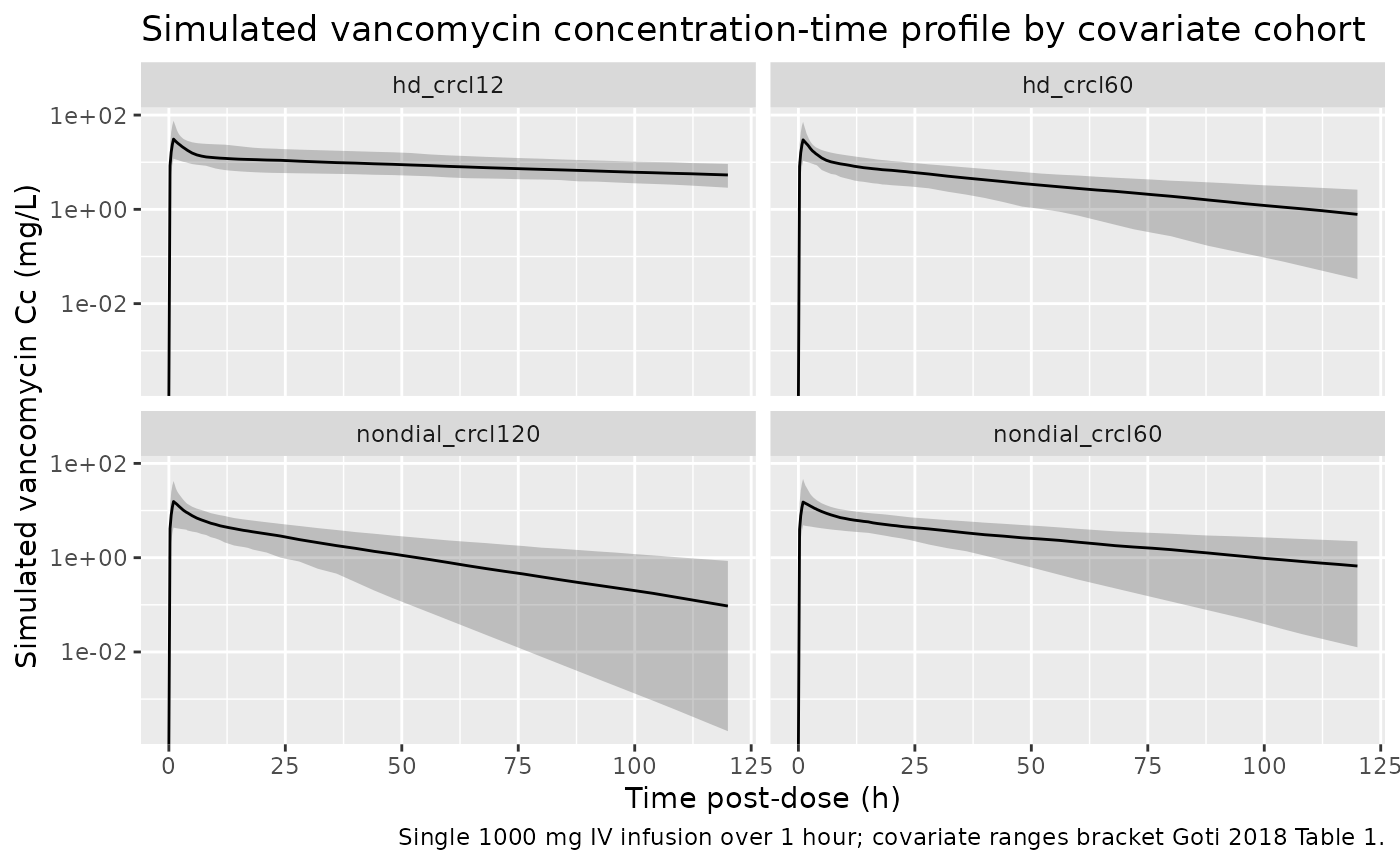
PKNCA validation
Goti 2018 does not publish single-dose NCA tables, so the PKNCA block
below characterises Cmax, Tmax, AUC0-inf, and half-life for each cohort
to give a one-table audit of the simulated PK. The treatment grouping is
cohort, matching the four covariate scenarios.
sim_nca <- sim |>
  filter(!is.na(Cc)) |>
  select(id, time, Cc, cohort)

dose_df <- events |>
  filter(evid == 1) |>
  select(id, time, amt, cohort)

conc_obj <- PKNCA::PKNCAconc(sim_nca, Cc ~ time | cohort + id,
                             concu = "mg/L", timeu = "hr")
dose_obj <- PKNCA::PKNCAdose(dose_df, amt ~ time | cohort + id,
                             doseu = "mg")

intervals <- data.frame(
  start       = 0,
  end         = Inf,
  cmax        = TRUE,
  tmax        = TRUE,
  aucinf.obs  = TRUE,
  half.life   = TRUE,
  clast.obs   = TRUE,
  lambda.z    = TRUE
)

nca_res <- PKNCA::pk.nca(
  PKNCA::PKNCAdata(conc_obj, dose_obj, intervals = intervals)
)

nca_summary <- summary(nca_res)
knitr::kable(nca_summary, caption = "Simulated NCA parameters by covariate cohort (single 1000 mg IV infusion over 1 hour).")| Interval Start | Interval End | cohort | N | Cmax (mg/L) | Tmax (hr) | Clast (mg/L) | Half-life (hr) | (1/hr) | AUCinf,obs (hr*mg/L) |
|---|---|---|---|---|---|---|---|---|---|
| 0 | Inf | hd_crcl12 | 200 | 30.0 [72.7] | 1.00 [1.00, 1.00] | 5.08 [48.3] | 124 [85.1] | 0.00668 [65.5] | 2020 [38.5] |
| 0 | Inf | hd_crcl60 | 200 | 26.8 [62.8] | 1.00 [1.00, 1.00] | 0.469 [404] | 37.0 [23.6] | 0.0223 [64.2] | 543 [39.8] |
| 0 | Inf | nondial_crcl120 | 200 | 16.4 [76.5] | 1.00 [1.00, 1.00] | 0.0378 [6860] | 22.2 [13.9] | 0.0369 [63.8] | 223 [39.9] |
| 0 | Inf | nondial_crcl60 | 200 | 14.4 [73.2] | 1.00 [1.00, 1.00] | 0.415 [300] | 39.7 [27.0] | 0.0207 [62.7] | 398 [36.8] |
Comparison against published Vss
Goti 2018 reports steady-state volume of distribution as 1.4 L/kg in the non-dialysis population and 1.0 L/kg in the dialysis population (Discussion paragraph 1). The packaged model recovers these values exactly from typical-value (Vc + Vp) computed at the WT = 70 kg reference.
vss_check <- tibble(
  cohort       = c("nondial_crcl120", "nondial_crcl60", "hd_crcl60", "hd_crcl12"),
  hemodial     = c(0, 0, 1, 1),
  vc_typical_L = 58.4 * c(1, 1, 0.5, 0.5),
  vp_typical_L = 38.4,
  vss_L_per_kg = (vc_typical_L + vp_typical_L) / 70,
  paper_vss    = c(1.4, 1.4, 1.0, 1.0)
)
knitr::kable(vss_check, caption = "Vss = (Vc + Vp) / WT at WT = 70 kg vs Goti 2018 reported values.")| cohort | hemodial | vc_typical_L | vp_typical_L | vss_L_per_kg | paper_vss |
|---|---|---|---|---|---|
| nondial_crcl120 | 0 | 58.4 | 38.4 | 1.3828571 | 1.4 |
| nondial_crcl60 | 0 | 58.4 | 38.4 | 1.3828571 | 1.4 |
| hd_crcl60 | 1 | 29.2 | 38.4 | 0.9657143 | 1.0 |
| hd_crcl12 | 1 | 29.2 | 38.4 | 0.9657143 | 1.0 |
Assumptions and deviations
- Vp WT scaling. Goti 2018 Table 2 displays the covariate equation TVVc = theta4 * (WT/70) * theta5^DIAL but does not show an explicit equation for TVVp. The Methods state that “volume parameters were normalized to a 70-kg individual” (plural, applying to both volumes), so the packaged model applies the same fixed-linear (WT/70) factor to Vp. Removing the Vp WT scaling has a small numerical effect on Vss at non-median weights but matches the prose less faithfully.
- RRT_HEMODIAL_STATUS is time-fixed. Goti 2018 used DIAL as a subject-level binary indicator because actual hemodialysis-session timestamps were not used (per Discussion limitations: “Limitations in the documentation prevented the usage of actual hemodialysis times”). The packaged model carries this assumption forward: drug removal during a dialysis session is not represented; the indicator captures the bulk PK shift in subjects who were chronically on intermittent hemodialysis during the admission.
-
CRCL preprocessing rules apply upstream of the
model. Goti 2018 truncated CRCL values >150 mL/min to 150
and reset SCr <1 mg/dL to 1 for subjects older than 60 years before
computing CrCL. The packaged model assumes the user has applied these
data-preparation rules before feeding CRCL into the simulation; the
covariateData[[CRCL]]notes restate the rules. - Final-model minimization status. Goti 2018 Results paragraph 2 states “The final model had a terminated minimization due to rounding errors and a successful covariance step (S-matrix calculation). Careful evaluation of output from the covariance step was conducted to accept the results. All the correlations between parameters were <0.95 in the correlation matrix.” The packaged parameter values are the explicitly-accepted final-model estimates from Table 2; the rounding-errors-but-covariance-accepted status is documented here for reproducibility but does not affect how the typical-value model is used.
- Q has no IIV in the source paper. Table 2 reports BSV%CV on CL, Vc, and Vp only. The packaged model leaves Q as a typical-value parameter with no eta, matching the published structure.
- Race / ethnicity distribution. Not reported by Goti 2018 (the data come from two academic medical centers serving a population with high prevalence of end-stage renal disease but no race / ethnic breakdown is given). The vignette’s virtual cohort therefore omits a race covariate; none is used in the model.