Dobutamine in neonates: PK and haemodynamic PD (Hallik 2020)
Source:vignettes/articles/Hallik_2020_dobutamine.Rmd
Hallik_2020_dobutamine.RmdModel and source
Hallik et al. (2020) studied dobutamine in 28 critically ill preterm and term neonates in their first 72 hours of life. They first fitted a population PK model to the plasma concentrations alone (Table 2), then fitted six separate simultaneous PKPD models, one per haemodynamic endpoint (Tables 4 and 5). Each PKPD fit re-estimated the PK parameters jointly with its endpoint while holding the maturation parameters fixed at their PK-only values. Following the authors’ structure, the library carries seven models:
| Model | Endpoint | PD form | Source |
|---|---|---|---|
Hallik_2020_dobutamine |
plasma concentration only | none | Table 2 |
Hallik_2020_dobutamine_rvo |
right ventricular output (rvo, mL/kg/min) |
linear in plasma C | Table 4 |
Hallik_2020_dobutamine_lvo |
left ventricular output (lvo, mL/kg/min) |
sigmoidal Emax in plasma C | Table 4 |
Hallik_2020_dobutamine_lvef |
left ventricular ejection fraction (lvef, %) |
linear in plasma C | Table 4 |
Hallik_2020_dobutamine_hr |
heart rate (hr, beats/min) |
sigmoidal Emax in effect-site C | Table 5 |
Hallik_2020_dobutamine_map |
mean arterial pressure (map, mmHg) |
sigmoidal Emax in plasma C | Table 5 |
Hallik_2020_dobutamine_ftoe_cerebral |
cerebral fractional tissue O2 extraction
(ftoe_cerebral) |
sigmoidal Emax in plasma C | Table 5 |
- Citation: Hallik M, Ilmoja M-L, Standing JF, Soeorg H, Jalas T, Raidmae M, Uibo K, Kobas K, Sonajalg M, Takkis K, Veigure R, Kipper K, Starkopf J, Metsvaht T. Population pharmacokinetics and pharmacodynamics of dobutamine in neonates on the first days of life. Br J Clin Pharmacol. 2020;86(2):318-328. doi:10.1111/bcp.14146.
- Description (PK model): One-compartment population PK model for intravenous dobutamine in critically ill preterm and term neonates in the first 3 days of life, given as a continuous infusion titrated from 5 to at most 20 ug/kg/min (Hallik 2020, final linear PK model of Table 2). Clearance is allometrically scaled to birth weight with a fixed exponent of 0.75 and multiplied by a sigmoidal postmenstrual-age maturation function (PMA50 = 37.4 weeks, Hill = 2.67); volume scales linearly with birth weight. Both are referenced to the 1618 g cohort median birth weight. Clearance and volume share a single random effect, which enters volume multiplied by an estimated scale factor of 1.34. Residual error is proportional (58.1%). The six simultaneous PKPD models the paper fitted on top of this PK structure (right and left ventricular output, ejection fraction, heart rate, mean arterial pressure, cerebral fractional tissue oxygen extraction) are the companion Hallik_2020_dobutamine_* models.
- Article: https://doi.org/10.1111/bcp.14146 (open access, PMC7015735)
Population
The analysis included 28 of 31 recruited neonates from two Estonian NICUs (Tallinn Children’s Hospital and Tartu University Hospital), April 2016 to December 2017. Table 1 gives gestational age at birth as median 30.4 weeks (range 22.7-41.0), with 25% below 28 weeks, 32% at 28-32 weeks, 25% at 32-37 weeks and 18% above 37 weeks; birth weight median 1618 g (465-4380 g); 64% male; and age at recruitment median 6 h (2-28 h). The main diagnoses were respiratory distress syndrome, early-onset sepsis, perinatal asphyxia, meconium aspiration and foeto-foetal transfusion. Dobutamine was infused from 5 ug/kg/min and raised by 5 ug/kg/min about every 30 minutes, up to 20 ug/kg/min. The highest dose reached was 10, 15 and 20 ug/kg/min in 1, 17 and 10 neonates. There were 119 plasma samples, 9 of them below the 0.97 ug/L LLOQ.
The same information is available programmatically via the
population element of each model, e.g.
rxode2::rxode(readModelDb("Hallik_2020_dobutamine"))$population.
Source trace
Every ini() value carries an in-file comment naming its
table row. The structure shared by all seven models is:
| Equation | Form in the model | Source location |
|---|---|---|
| CL | exp(lcl + etalcl) * (WT_BIRTH/1.618)^0.75 * PAGE^hill_mat / (tmat50^hill_mat + PAGE^hill_mat) |
Equation 1 |
| V | exp(lvc + vc_eta_scale * etalcl) * (WT_BIRTH/1.618) |
Equation 2; Methods 2.3 (shared BSV with scale factor on V) |
| Effect site (HR only) | d/dt(effect) <- ke0 * (Cc - effect) |
Equation 3 |
| Linear PD (RVO, LVEF) | E = rbase + slope * C |
Equation 4 |
| Sigmoidal Emax PD (LVO, HR, MAP, cFTOE) | E = rbase + (rmax - rbase) * C^hill / (ec50^hill + C^hill) |
Equation 6 |
| BSV scale | omega2 = (CV/100)^2 | Tables 2, 4, 5 footnote a: CV = sqrt(omega2) x 100% |
| Residual error | proportional on every output | Results 3.1 |
The PK part of each model:
| Model |
lcl (L/h per 1618 g) |
lvc (L per 1618 g) |
vc_eta_scale |
tmat50 (weeks) |
hill_mat |
CL BSV | PK propSd
|
Source |
|---|---|---|---|---|---|---|---|---|
| PK only | 41.2 | 5.29 | 1.34 | 37.4 | 2.67 | 29% | 0.581 | Table 2 |
| RVO | 41.0 | 5.31 | 1.50 | 37.4 fixed | 2.67 fixed | 27% | 0.583 | Table 4 |
| LVO | 40.7 | 5.14 | 1.33 | 37.4 fixed | 2.67 fixed | 25% | 0.589 | Table 4 |
| LVEF | 41.2 | 5.26 | 1.38 | 37.4 fixed | 2.67 fixed | 28% | 0.580 | Table 4 |
| HR | 42.3 | 5.42 | 1.72 | 37.4 fixed | 2.67 fixed | 27% | 0.590 | Table 5 |
| MAP | 37.2 | 4.88 | 3.62 | 37.4 fixed | 2.67 fixed | 24% | 0.675 | Table 5 |
| cFTOE | 37.2 | 4.80 | 2.42 | 37.4 fixed | 2.67 fixed | 35% | 0.653 | Table 5 |
The allometric exponent 0.75 on CL is fixed in every model (Equation 1 prints it as a literal). The PD part of each model (BSV as CV in parentheses; “-” = not estimated):
| Model | E0 (rbase) |
Slope / Emax (slope / rmax) |
EC50 (ug/L) | Hill | keo (1/h) | PD propSd
|
Source |
|---|---|---|---|---|---|---|---|
| RVO | 151 mL/kg/min (41%) | SL 0.214 | - | - | - | 0.184 | Table 4 |
| LVO | 131 mL/kg/min (36%) | Emax 157 mL/kg/min (44%) | 117 | 2.82 | - | 0.167 | Table 4 |
| LVEF | 63.5% (9%) | SL 0.0285 | - | - | - | 0.098 | Table 4 |
| HR | 138 /min (15%) | Emax 172 /min (5%) | 39.2 (50%) | 3.36 | 6.59 | 0.051 | Table 5 |
| MAP | 39.7 mmHg (22%) | Emax 41.9 mmHg (26%) | 25.4 | 13.5 | - | 0.065 | Table 5 |
| cFTOE | 0.227 (50%) | Emax 0.206 (60%) | 52.9 | 3.65 | - | 0.181 | Table 5 |
Virtual cohort
Individual data are not published. The cohort below reproduces the Table 1 gestational-age bands. Birth weight is drawn around an approximate 50th-percentile birth weight for gestational age (log-normal, SD 0.15 on the log scale). Postmenstrual age is the gestational age plus 6 hours, the median age at recruitment.
set.seed(2020)
rxode2::rxSetSeed(2020)
n_sub <- 200

# Approximate 50th-percentile birth weight (kg) by gestational age (weeks);
# used only to give the virtual cohort a realistic GA-weight correlation.
bw50 <- data.frame(
  ga = c(22, 24, 26, 28, 30, 32, 34, 36, 38, 40, 42),
  bw = c(0.50, 0.65, 0.90, 1.15, 1.45, 1.80, 2.25, 2.70, 3.10, 3.45, 3.65)
)

make_cohort <- function(n) {
  band <- sample(1:4, n, replace = TRUE, prob = c(0.25, 0.32, 0.25, 0.18))
  lo <- c(22.7, 28, 32, 37)[band]
  hi <- c(28, 32, 37, 41.0)[band]
  ga <- stats::runif(n, lo, hi)
  bw <- stats::approx(bw50$ga, bw50$bw, xout = ga)$y * exp(stats::rnorm(n, 0, 0.15))
  data.frame(
    id = seq_len(n),
    GA = ga,
    WT_BIRTH = pmin(pmax(bw, 0.465), 4.38),
    PAGE = ga + 6 / (24 * 7)
  )
}
cohort <- make_cohort(n_sub)

cohort |>
  summarise(
    `GA median (weeks)` = median(GA),
    `GA range` = paste(round(range(GA), 1), collapse = "-"),
    `Birth weight median (kg)` = median(WT_BIRTH),
    `Birth weight range` = paste(round(range(WT_BIRTH), 2), collapse = "-")
  ) |>
knitr::kable(digits = 2, caption = "Virtual cohort (compare Table 1: GA 30.4, 22.7-41.0 weeks; BW 1.618, 0.465-4.38 kg).")| GA median (weeks) | GA range | Birth weight median (kg) | Birth weight range |
|---|---|---|---|
| 31.2 | 22.7-40.9 | 1.7 | 0.47-4.38 |
Dosing
The simulated regimen follows the study protocol (Methods 2.1): 5
ug/kg/min from time zero, raised by 5 ug/kg/min every 30 minutes to 20
ug/kg/min, which is held until 3 h, followed by 1 h of washout. With
dose in ug and time in hours, an infusion of R ug/kg/min enters
central at a rate of R * WT_BIRTH * 60
ug/h.
steps <- data.frame(
  start = c(0, 0.5, 1, 1.5),
  end = c(0.5, 1, 1.5, 3),
  dose_rate = c(5, 10, 15, 20)
)

make_events <- function(cohort, steps, obs_times) {
  doses <- tidyr::crossing(cohort, steps) |>
    mutate(
      time = start,
      evid = 1L,
      cmt = "central",
      rate = dose_rate * WT_BIRTH * 60,
      amt = rate * (end - start)
    ) |>
    select(id, time, evid, cmt, amt, rate, WT_BIRTH, PAGE)
  obs <- tidyr::crossing(cohort, time = obs_times) |>
    mutate(evid = 0L, cmt = "central", amt = NA_real_, rate = NA_real_) |>
    select(id, time, evid, cmt, amt, rate, WT_BIRTH, PAGE)
  bind_rows(doses, obs) |> arrange(id, time, desc(evid))
}

obs_times <- sort(unique(c(seq(0, 4, by = 2 / 60), c(0.5, 1, 1.5, 3) - 1 / 60)))
ev <- make_events(cohort, steps, obs_times)
Dobutamine concentrations
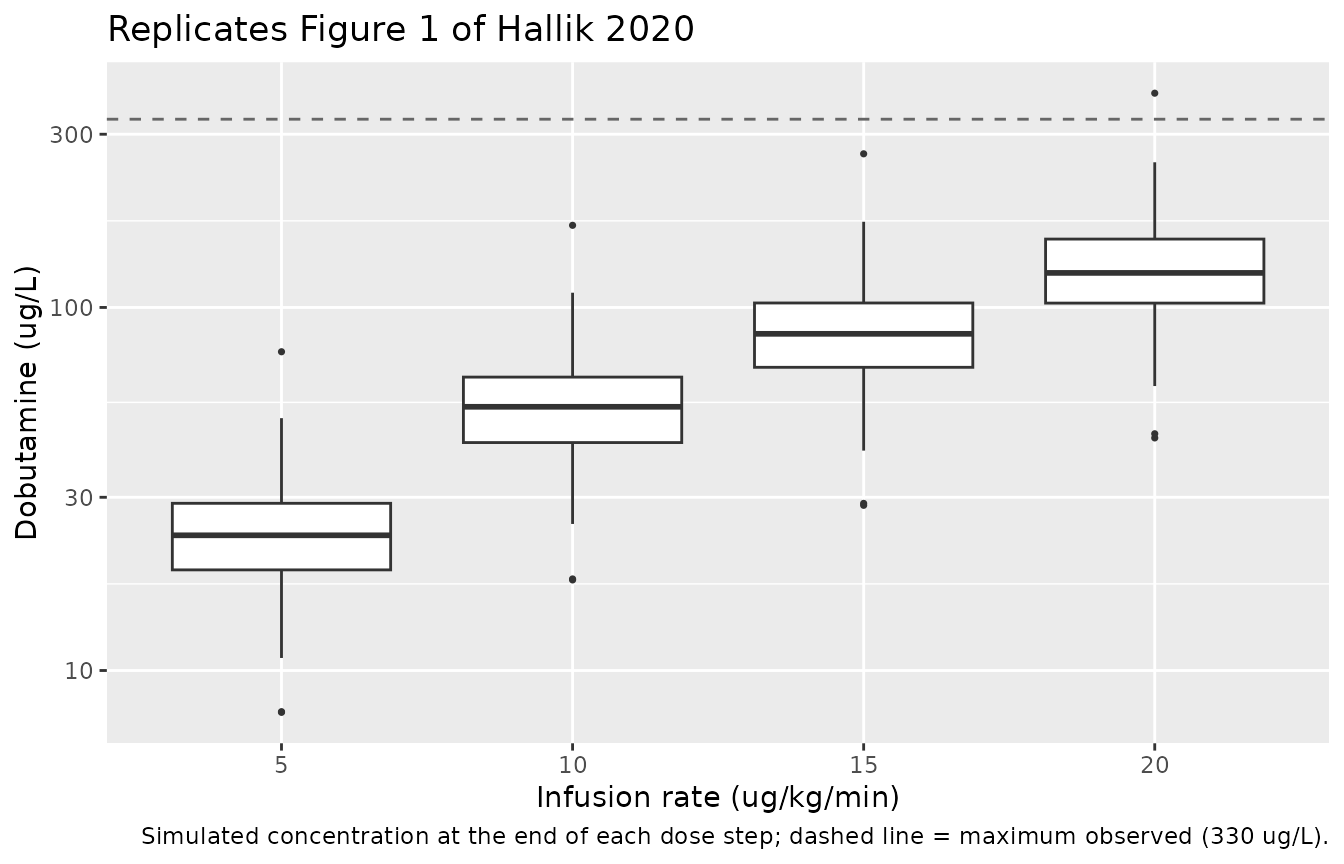
Concentration against infusion rate (Figure 1)
Figure 1 plots each measured concentration against the infusion rate running at the time. Samples were drawn 15-30 min after each dose change. The simulation below reads the concentration one minute before each step ends. The paper’s maximum measured concentration was 330 ug/L.
mod_pk <- rxode2::rxode(readModelDb("Hallik_2020_dobutamine"))
#> ℹ parameter labels from comments will be replaced by 'label()'
sim_pk <- rxode2::rxSolve(mod_pk, events = ev, keep = c("WT_BIRTH", "PAGE")) |>
  as.data.frame()

step_ends <- data.frame(
  time = c(0.5, 1, 1.5, 3) - 1 / 60,
  dose_rate = c(5, 10, 15, 20)
)
conc_by_rate <- sim_pk |>
  inner_join(step_ends, by = "time")

ggplot(conc_by_rate, aes(factor(dose_rate), Cc)) +
  geom_boxplot(outlier.size = 0.6) +
  geom_hline(yintercept = 330, linetype = "dashed", colour = "grey40") +
  scale_y_log10() +
  labs(
    x = "Infusion rate (ug/kg/min)", y = "Dobutamine (ug/L)",
    title = "Replicates Figure 1 of Hallik 2020",
    caption = "Simulated concentration at the end of each dose step; dashed line = maximum observed (330 ug/L)."
  )
conc_by_rate |>
  group_by(`Infusion rate (ug/kg/min)` = dose_rate) |>
  summarise(
    `Median (ug/L)` = median(Cc),
    `5th pct` = quantile(Cc, 0.05),
    `95th pct` = quantile(Cc, 0.95),
    .groups = "drop"
  ) |>
knitr::kable(digits = 1)| Infusion rate (ug/kg/min) | Median (ug/L) | 5th pct | 95th pct |
|---|---|---|---|
| 5 | 23.6 | 12.5 | 39.1 |
| 10 | 53.3 | 28.6 | 86.4 |
| 15 | 84.6 | 45.2 | 138.2 |
| 20 | 124.5 | 68.7 | 200.8 |
The median concentration rises about in proportion to the infusion rate, as Figure 1 shows for the observed data. The simulated 95th percentile at 20 ug/kg/min is of the same order as the 330 ug/L maximum observed.
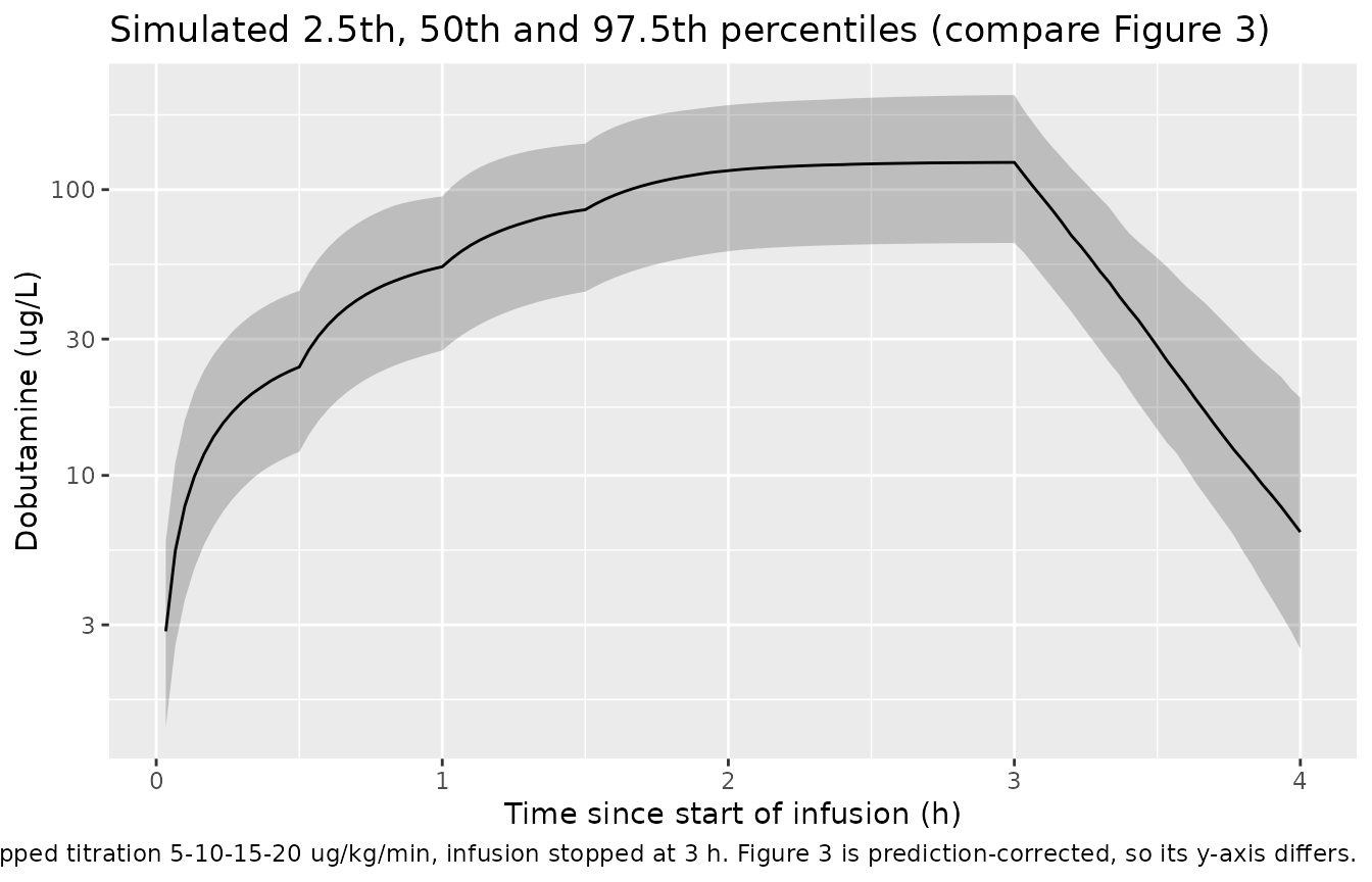
Concentration-time profile (Figure 3)
# Drop t = 0 (Cc = 0) only because the axis is logarithmic.
sim_pk[sim_pk$time > 0, ] |>
  group_by(time) |>
  summarise(
    p025 = quantile(Cc, 0.025), p50 = median(Cc), p975 = quantile(Cc, 0.975),
    .groups = "drop"
  ) |>
  ggplot(aes(time, p50)) +
  geom_ribbon(aes(ymin = p025, ymax = p975), alpha = 0.25) +
  geom_line() +
  scale_y_log10() +
  labs(
    x = "Time since start of infusion (h)", y = "Dobutamine (ug/L)",
    title = "Simulated 2.5th, 50th and 97.5th percentiles (compare Figure 3)",
    caption = "Stepped titration 5-10-15-20 ug/kg/min, infusion stopped at 3 h. Figure 3 is prediction-corrected, so its y-axis differs."
  )
Typical-value checks against the text
The Discussion reports that the typical volume of 5.29 L per 1618 g
is 3.27 L/kg. The maturation function gives the typical clearance at the
cohort’s median postmenstrual age. The mean effect-equilibration time
for heart rate (Results 3.1) is 60 / keo.
th <- rxode2::rxode(readModelDb("Hallik_2020_dobutamine"))$theta
#> ℹ parameter labels from comments will be replaced by 'label()'
fmat <- function(pma, tm50, hill) pma^hill / (tm50^hill + pma^hill)
v_per_kg <- exp(th[["lvc"]]) / 1.618
cl_typ <- exp(th[["lcl"]]) * fmat(30.4, exp(th[["ltmat50"]]), exp(th[["lhill_mat"]]))
thalf_min <- log(2) * exp(th[["lvc"]]) / cl_typ * 60
th_hr <- rxode2::rxode(readModelDb("Hallik_2020_dobutamine_hr"))$theta
#> ℹ parameter labels from comments will be replaced by 'label()'
mean_eq_time <- 60 / exp(th_hr[["lke0"]])

data.frame(
  Quantity = c(
    "V per kg (L/kg)", "Typical CL at PMA 30.4 weeks (L/h per 1618 g)",
    "Typical CL at PMA 30.4 weeks (mL/min/kg)", "Typical half-life (min)",
    "HR mean equilibration time (min)"
  ),
  Model = c(v_per_kg, cl_typ, cl_typ / 1.618 * 1000 / 60, thalf_min, mean_eq_time),
  Paper = c("3.27 (Discussion 4.1)", "-", "-", "-", "9 (Results 3.1)")
) |>
knitr::kable(digits = 2)| Quantity | Model | Paper |
|---|---|---|
| V per kg (L/kg) | 3.27 | 3.27 (Discussion 4.1) |
| Typical CL at PMA 30.4 weeks (L/h per 1618 g) | 15.04 | - |
| Typical CL at PMA 30.4 weeks (mL/min/kg) | 154.95 | - |
| Typical half-life (min) | 14.63 | - |
| HR mean equilibration time (min) | 9.10 | 9 (Results 3.1) |
PKNCA validation
To check the PK model with an independent method, three arms of 100 virtual neonates receive a constant 4-hour infusion of 5, 10 or 20 ug/kg/min, followed by 2 hours of washout. PKNCA estimates clearance as dose / AUC0-inf. Because the model is linear, this should recover each subject’s own model clearance. Any difference is trapezoidal integration error, not a model property.
nca_cohort <- make_cohort(300) |>
  mutate(treatment = rep(c("5 ug/kg/min", "10 ug/kg/min", "20 ug/kg/min"), each = 100),
         dose_rate = rep(c(5, 10, 20), each = 100))

nca_doses <- nca_cohort |>
  mutate(time = 0, evid = 1L, cmt = "central", rate = dose_rate * WT_BIRTH * 60,
         amt = rate * 4, dur = 4)
nca_obs <- tidyr::crossing(nca_cohort, time = sort(unique(c(seq(0, 6, by = 0.05), 4)))) |>
  mutate(evid = 0L, cmt = "central", amt = NA_real_, rate = NA_real_)
ev_nca <- bind_rows(
  select(nca_doses, id, time, evid, cmt, amt, rate, WT_BIRTH, PAGE, treatment),
  select(nca_obs, id, time, evid, cmt, amt, rate, WT_BIRTH, PAGE, treatment)
) |>
  arrange(id, time, desc(evid))

sim_nca <- rxode2::rxSolve(mod_pk, events = ev_nca, keep = c("treatment"),
                           rtol = 1e-10, atol = 1e-12) |>
  as.data.frame()

conc_nca <- sim_nca |>
  filter(!is.na(Cc)) |>
  mutate(Cc = pmax(Cc, 0)) |>
  select(id, time, Cc, treatment)
conc_nca <- bind_rows(
  conc_nca,
  conc_nca |> distinct(id, treatment) |> mutate(time = 0, Cc = 0)
) |>
  distinct(id, treatment, time, .keep_all = TRUE) |>
  arrange(id, treatment, time)

conc_obj <- PKNCA::PKNCAconc(conc_nca, Cc ~ time | treatment + id)
dose_obj <- PKNCA::PKNCAdose(
  select(nca_doses, id, time, amt, dur, treatment),
  amt ~ time | treatment + id,
  route = "intravascular", duration = "dur"
)
intervals <- data.frame(
  start = 0, end = Inf,
  cmax = TRUE, aucinf.obs = TRUE, cl.obs = TRUE, half.life = TRUE
)
nca_res <- PKNCA::pk.nca(PKNCA::PKNCAdata(conc_obj, dose_obj, intervals = intervals))

nca_wide <- as.data.frame(nca_res) |>
  filter(PPTESTCD %in% c("cmax", "cl.obs", "half.life")) |>
  select(id, treatment, PPTESTCD, PPORRES) |>
  tidyr::pivot_wider(names_from = PPTESTCD, values_from = PPORRES)

model_cl <- sim_nca |>
  group_by(id) |>
  summarise(cl_model = first(cl), vc_model = first(vc), .groups = "drop")

nca_check <- nca_wide |>
  left_join(model_cl, by = "id") |>
  mutate(
    pct_diff_cl = 100 * (cl.obs / cl_model - 1),
    thalf_model = log(2) * vc_model / cl_model
  )

nca_check |>
  group_by(treatment) |>
  summarise(
    `Median Cmax (ug/L)` = median(cmax),
    `Median CL, PKNCA (L/h)` = median(cl.obs),
    `Median CL, model (L/h)` = median(cl_model),
    `Median t1/2, PKNCA (min)` = median(half.life) * 60,
    `Median t1/2, model (min)` = median(thalf_model) * 60,
    .groups = "drop"
  ) |>
knitr::kable(digits = 2, caption = "PKNCA against each subject's own model parameters, by infusion arm.")| treatment | Median Cmax (ug/L) | Median CL, PKNCA (L/h) | Median CL, model (L/h) | Median t1/2, PKNCA (min) | Median t1/2, model (min) |
|---|---|---|---|---|---|
| 10 ug/kg/min | 60.95 | 17.31 | 17.31 | 13.94 | 13.94 |
| 20 ug/kg/min | 125.87 | 17.01 | 17.01 | 13.77 | 13.77 |
| 5 ug/kg/min | 30.93 | 18.32 | 18.31 | 13.92 | 13.92 |
# Same-parameter check: dose/AUC against the subject's own CL, so the only gap
# is trapezoidal error on a 3-minute grid (washout t1/2 ~ 5-40 min).
stopifnot(
  abs(median(nca_check$pct_diff_cl)) < 2,
  quantile(abs(nca_check$pct_diff_cl), 0.9) < 5
)
The paper reports no NCA of its own data, so there is no published table to compare against. Clearance does not change with the infusion rate, which matches the paper’s finding that dobutamine PK was linear over 5-20 ug/kg/min (Results 3.1).
Haemodynamic endpoints
Typical concentration-effect curves
Each endpoint’s typical-value concentration-effect relationship, evaluated over the observed concentration range (up to 330 ug/L). For heart rate the driver is the effect-site concentration, which equals the plasma concentration at steady state.
theta_of <- function(name) rxode2::rxode(readModelDb(name))$theta
emax_curve <- function(conc, th, sfx) {
  e0 <- exp(th[[paste0("lrbase_", sfx)]])
  emax <- exp(th[[paste0("lrmax_", sfx)]])
  ec50 <- exp(th[[paste0("lec50_", sfx)]])
  hill <- exp(th[[paste0("lhill_", sfx)]])
  e0 + (emax - e0) * conc^hill / (ec50^hill + conc^hill)
}
linear_curve <- function(conc, th, sfx) {
  exp(th[[paste0("lrbase_", sfx)]]) + exp(th[[paste0("lslope_", sfx)]]) * conc
}

conc_grid <- seq(0, 330, by = 1)
ce <- bind_rows(
  data.frame(endpoint = "RVO (mL/kg/min)", conc = conc_grid,
             effect = linear_curve(conc_grid, theta_of("Hallik_2020_dobutamine_rvo"), "rvo")),
  data.frame(endpoint = "LVO (mL/kg/min)", conc = conc_grid,
             effect = emax_curve(conc_grid, theta_of("Hallik_2020_dobutamine_lvo"), "lvo")),
  data.frame(endpoint = "LVEF (%)", conc = conc_grid,
             effect = linear_curve(conc_grid, theta_of("Hallik_2020_dobutamine_lvef"), "lvef")),
  data.frame(endpoint = "HR (beats/min)", conc = conc_grid,
             effect = emax_curve(conc_grid, theta_of("Hallik_2020_dobutamine_hr"), "hr")),
  data.frame(endpoint = "MAP (mmHg)", conc = conc_grid,
             effect = emax_curve(conc_grid, theta_of("Hallik_2020_dobutamine_map"), "map")),
  data.frame(endpoint = "cFTOE", conc = conc_grid,
             effect = emax_curve(conc_grid, theta_of("Hallik_2020_dobutamine_ftoe_cerebral"), "ftoe_cerebral"))
)
#> ℹ parameter labels from comments will be replaced by 'label()'
#> ℹ parameter labels from comments will be replaced by 'label()'
#> ℹ parameter labels from comments will be replaced by 'label()'
#> ℹ parameter labels from comments will be replaced by 'label()'
#> ℹ parameter labels from comments will be replaced by 'label()'
#> ℹ parameter labels from comments will be replaced by 'label()'

ggplot(ce, aes(conc, effect)) +
  geom_line() +
  facet_wrap(~endpoint, scales = "free_y") +
  labs(x = "Dobutamine concentration (ug/L)", y = "Typical endpoint value",
       title = "Typical concentration-effect relationships (Tables 4 and 5)")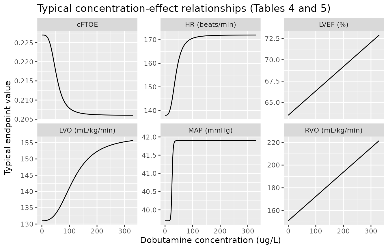
The Discussion makes several claims about these curves. Mean heart rate rises from 138 to 172 beats/min. The MAP and HR effects reach their maximum “within concentrations of 50 and 80 ug/L, respectively”. LVO keeps rising “at least up to concentration of 200 ug/L”. cFTOE falls with dobutamine. The fraction of each maximal change reached at those concentrations is checked below.
frac_of_max <- function(conc, th, sfx) {
  e0 <- exp(th[[paste0("lrbase_", sfx)]])
  (emax_curve(conc, th, sfx) - e0) / (exp(th[[paste0("lrmax_", sfx)]]) - e0)
}
th_map <- theta_of("Hallik_2020_dobutamine_map")
#> ℹ parameter labels from comments will be replaced by 'label()'
th_lvo <- theta_of("Hallik_2020_dobutamine_lvo")
#> ℹ parameter labels from comments will be replaced by 'label()'
th_ftoe <- theta_of("Hallik_2020_dobutamine_ftoe_cerebral")
#> ℹ parameter labels from comments will be replaced by 'label()'

checks <- data.frame(
  Claim = c(
    "HR baseline -> maximum (beats/min)",
    "MAP: fraction of maximal change at 50 ug/L",
    "HR: fraction of maximal change at 80 ug/L",
    "LVO: fraction of maximal change at 200 ug/L",
    "cFTOE change at 330 ug/L (typical)"
  ),
  Model = c(
    sprintf("%.0f -> %.0f", exp(th_hr[["lrbase_hr"]]), exp(th_hr[["lrmax_hr"]])),
    sprintf("%.3f", frac_of_max(50, th_map, "map")),
    sprintf("%.3f", frac_of_max(80, th_hr, "hr")),
    sprintf("%.3f", frac_of_max(200, th_lvo, "lvo")),
    sprintf("%+.3f", emax_curve(330, th_ftoe, "ftoe_cerebral") - exp(th_ftoe[["lrbase_ftoe_cerebral"]]))
  )
)
knitr::kable(checks)| Claim | Model |
|---|---|
| HR baseline -> maximum (beats/min) | 138 -> 172 |
| MAP: fraction of maximal change at 50 ug/L | 1.000 |
| HR: fraction of maximal change at 80 ug/L | 0.917 |
| LVO: fraction of maximal change at 200 ug/L | 0.819 |
| cFTOE change at 330 ug/L (typical) | -0.021 |
Endpoint time courses under the titration (Figure 4)
Figure 4 shows prediction-corrected VPCs of each endpoint over time.
The simulation below applies the stepped titration to the virtual cohort
for each of the six PKPD models. It shows the median and 95% interval of
each endpoint. Each PKPD model has two outputs, the concentration and
the endpoint, and neither is an ODE state. The observation rows are
therefore keyed by dvid = 1 with no compartment, and rxode2
returns both output columns at every observation time.
pd_models <- c(
  rvo = "Hallik_2020_dobutamine_rvo", lvo = "Hallik_2020_dobutamine_lvo",
  lvef = "Hallik_2020_dobutamine_lvef", hr = "Hallik_2020_dobutamine_hr",
  map = "Hallik_2020_dobutamine_map", ftoe_cerebral = "Hallik_2020_dobutamine_ftoe_cerebral"
)
pd_labels <- c(
  rvo = "RVO (mL/kg/min)", lvo = "LVO (mL/kg/min)", lvef = "LVEF (%)",
  hr = "HR (beats/min)", map = "MAP (mmHg)", ftoe_cerebral = "cFTOE"
)

ev_pd <- ev |>
  mutate(
    dvid = ifelse(evid == 0L, 1L, NA_integer_),
    cmt = ifelse(evid == 0L, NA_character_, cmt)
  )

sim_pd <- lapply(names(pd_models), function(out) {
  mod <- rxode2::rxode(readModelDb(pd_models[[out]]))
  s <- rxode2::rxSolve(mod, events = ev_pd, useLinCmt = FALSE) |> as.data.frame()
  data.frame(id = s$id, time = s$time, endpoint = pd_labels[[out]], value = s[[out]])
}) |>
  bind_rows()
#> ℹ parameter labels from comments will be replaced by 'label()'
#> ℹ parameter labels from comments will be replaced by 'label()'
#> ℹ parameter labels from comments will be replaced by 'label()'
#> ℹ parameter labels from comments will be replaced by 'label()'
#> ℹ parameter labels from comments will be replaced by 'label()'
#> ℹ parameter labels from comments will be replaced by 'label()'

pd_summary <- sim_pd |>
  group_by(endpoint, time) |>
  summarise(
    p025 = quantile(value, 0.025), p50 = median(value), p975 = quantile(value, 0.975),
    .groups = "drop"
  )

ggplot(pd_summary, aes(time, p50)) +
  geom_ribbon(aes(ymin = p025, ymax = p975), alpha = 0.25) +
  geom_line() +
  geom_vline(xintercept = c(0.5, 1, 1.5, 3), linetype = "dotted", colour = "grey50") +
  facet_wrap(~endpoint, scales = "free_y") +
  labs(x = "Time since start of infusion (h)", y = "Endpoint value",
       title = "Simulated endpoint time courses (compare Figure 4)",
       caption = "Dotted lines: dose steps at 0.5, 1, 1.5 h and infusion stop at 3 h.")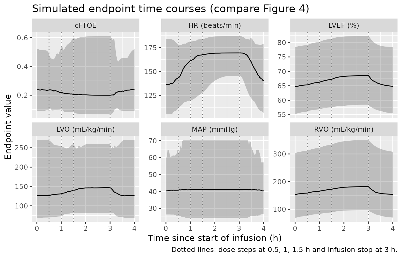
# Median endpoint at baseline and at the end of the 20 ug/kg/min step.
pd_table <- sim_pd |>
  filter(time %in% c(0, 3 - 1 / 60)) |>
  mutate(when = ifelse(time == 0, "Baseline", "End of 20 ug/kg/min")) |>
  group_by(endpoint, when) |>
  summarise(median = median(value), .groups = "drop") |>
  tidyr::pivot_wider(names_from = when, values_from = median)
knitr::kable(pd_table, digits = 3,
caption = "Median simulated endpoint before the infusion and at the top dose.")| endpoint | Baseline | End of 20 ug/kg/min |
|---|---|---|
| HR (beats/min) | 136.447 | 169.444 |
| LVEF (%) | 64.653 | 68.560 |
| LVO (mL/kg/min) | 126.642 | 147.087 |
| MAP (mmHg) | 40.369 | 41.159 |
| RVO (mL/kg/min) | 152.964 | 181.722 |
| cFTOE | 0.237 | 0.199 |
hr_top <- pd_table$`End of 20 ug/kg/min`[pd_table$endpoint == "HR (beats/min)"]
hr_base <- pd_table$Baseline[pd_table$endpoint == "HR (beats/min)"]
# Baseline medians are the E0 estimates (lognormal BSV: median = typical).
# Robust centre checks only (see the article's assumptions section).
stopifnot(
  abs(hr_base / 138 - 1) < 0.05,
  hr_top > hr_base,
  hr_top <= 172 * 1.05
)
Assumptions and deviations
- Model count. The paper reports one PK-only model and six separately fitted PKPD models, each with its own re-estimated PK parameters. All seven are carried as separate models, so a user picks the fit that matches the endpoint of interest. The six PKPD models describe the same drug but are not a single joint model.
-
Emax is a plateau level. Equations 5 and 6 write
E = E0 + (Emax - E0) * .... The paper defines Emax as “the estimated maximum HD parameter value”, so it is the plateau level, not the increment. The models therefore name itrmax_<endpoint>rather thanemax, followingDings_2026_cafedrine_theodrenaline_ephedrine. For cFTOE the plateau (0.206) lies below the baseline (0.227), so the effect is a fall, as the Discussion states. -
Shared random effect. Methods: “a shared BSV was
used with an estimated scale factor applied for V”. The single eta is
placed on CL and enters V multiplied by
vc_eta_scale. The tables print the same BSV value in the CL and V rows. We read that as the variance of the shared eta, so the implied CV of V is the scale factor times the CL CV (for example 1.34 x 29% = 39% in the PK-only model). - V exponent. Equation 2 prints no exponent on (BW/Wst), so V scales linearly with birth weight.
-
Birth weight as the size covariate. The paper
scales on birth weight. The models use
WT_BIRTHin kg with a 1.618 kg reference, which is the same ratio as the paper’s 1618 g. Infusion rates in ug/kg/min are converted with the same weight. -
PMA in weeks.
PAGEis declared in weeks, as the paper states it, rather than the register’s default of months. - Residual error. Every residual error is read as a proportional SD, not a variance. This fits the Results statement that residual variability was “>50% in PK observations and between 5-20% in PD observations”.
- BLQ handling. Concentrations below the 0.97 ug/L LLOQ were set to 0.5 ug/L in the fit (Methods 2.1). This affects estimation only, not the simulation model.
-
Covariates screened and not retained (Methods 2.3):
postnatal age, antenatal glucocorticoids, dopamine co-administration,
haemoglobin, albumin, patent ductus arteriosus diameter, baseline LVEF
and baseline RVO. Those with a canonical column are listed in
covariatesDataExcludedof the PK-only model. - Virtual cohort. Individual data are not published. The gestational-age bands follow Table 1. Birth weight for gestational age uses an approximate 50th-percentile curve with 15% log-scale spread. This is the maintainers’ approximation and only affects the spread of the simulated profiles, not the typical-value checks.
- No published NCA. The paper gives no Cmax, AUC or half-life summaries. The PKNCA section therefore checks the model against itself (dose/AUC against each subject’s clearance) rather than against published values.
- Errata. A search of Europe PMC and Crossref (September 2026) found no erratum or correction for this article.