Fentanyl in preterm and term newborns (Wu 2022)
Source:vignettes/articles/Wu_2022_fentanyl.Rmd
Wu_2022_fentanyl.RmdModel and source
- Citation: Wu Y, Voller S, Flint RB, Simons SHP, Allegaert K, Fellman V, Knibbe CAJ (2022). Pre- and Postnatal Maturation are Important for Fentanyl Exposure in Preterm and Term Newborns: A Pooled Population Pharmacokinetic Study. Clin Pharmacokinet 61(3):401-412. doi:10.1007/s40262-021-01076-0. Electronic supplementary material 1 (NONMEM control stream) used for the structural form, the dataset-indicator orientation and the residual-error scale.
- Description: Two-compartment intravenous population PK model for fentanyl in preterm and term newborns (164 neonates, gestational age 23.9-42.3 weeks, birth weight 0.39-4.245 kg, postnatal age 0-68 days) pooled from a Helsinki continuous-infusion study and the Dutch multicentre DINO study. Clearance is a product of two power functions, one of birth weight (prenatal maturation, centred on 1.055 kg) and one of postnatal age in days plus 0.01 (postnatal maturation, centred on 0.99 days). Central volume scales with current body weight through a bodyweight-dependent exponent (BDE) that itself falls as a power function of current weight, both centred on 1.165 kg. Intercompartmental clearance and peripheral volume carry no covariates. Log-normal IIV on clearance and central volume; separate combined additive and proportional residual errors for the two pooled datasets.
- Article: Clin Pharmacokinet 2022;61(3):401-412 (open access, PMC8891207). The electronic supplementary material (ESM) carries the final NONMEM control stream.
Wu and colleagues pooled 673 fentanyl plasma concentrations from 164 newborns across the whole neonatal range – gestational age 24 to 42 weeks – and fitted a two-compartment model in NONMEM 7.4. Clearance depends on two separate maturation processes: prenatal maturation, captured by birth weight, and postnatal maturation, captured by postnatal age. Combining the two was better than postmenstrual age alone (dOFV = -91). Central volume scales with current body weight through a bodyweight-dependent exponent (BDE). The weight exponent is itself a power function of weight, so volume changes fastest in the smallest neonates. The authors use the model to show that a flat 1 ug/kg/h infusion gives very different exposure across birth weight and postnatal age, and they propose a birth-weight and postnatal-age banded infusion regimen (their Table 3).
Population
The analysis data set (Wu 2022 Table 1) combines two studies.
- Dataset 1 (Helsinki). 66 mechanically ventilated newborns at the Hospital for Children and Adolescents, University of Helsinki (Saarenmaa 2000). The planned regimen was 10.5 ug/kg over 1 h, then a continuous infusion (median 1.5 ug/kg/h for a median 58 h). Arterial samples were taken at 2, 12, 24, 48 and 60 h. The assay was a radioimmunoassay with an LLOQ of 1 ug/L. Median gestational age 31.25 weeks (25.30-42.30), birth weight 1632 g (760-4245), postnatal age at the start of treatment 0.46 days. Current weight was not recorded and was set equal to birth weight.
- Dataset 2 (DINO). 98 preterm infants in four Dutch NICUs (the DINO study, NCT02421068). Physicians chose boluses of 0.5-3 ug/kg (median 2.1 ug/kg over 3 min) and/or infusions of 0.5-3 ug/kg/h. Samples were scavenged during routine care and assayed by LC-MS/MS with an LLOQ of 0.3 ug/L. Median gestational age 27.10 weeks (23.90-31.90), birth weight 906 g (390-1905), postnatal age 4.5 days (0-68).
Combined: 61.6% male; median gestational age 28.95 weeks; median
birth weight 1055 g; median current weight 1165 g; median postnatal age
1.1 days. The two medians, 1055 g and 1165 g, are the centring values of
the clearance and volume covariate models. The same information is in
readModelDb("Wu_2022_fentanyl") under
population.
Source trace
| Model element | Value | Source |
|---|---|---|
| Structure: two-compartment, IV input, first-order elimination | ADVAN3 TRANS4 | Results 3.1; ESM control stream $SUBROUTINES
|
lcl (TVCL) |
0.31 L/h | Table 2 |
e_wt_birth_cl (theta BW) |
1.47 | Table 2 (Eq. 2 in the text prints 1.57 – see below) |
e_pna_cl (theta PNA) |
0.505 | Table 2 (Eq. 2 prints 0.502) |
| CL = TVCL (BW/1055)^thetaBW (PNA+0.01)^thetaPNA | days, g | Eq. 2; Table 2 header row; ESM $PK
|
lvc (TVV1) |
10.6 L | Table 2 |
e_wt_vc (BDE intercept L1) |
1.56 | Table 2 |
bde_m_vc (BDE slope M) |
-0.417 | Table 2 |
| V1 = TVV1 (CW/1165)^BDE, BDE = L1 (CW/1165)^M | g | Eq. 3; Table 2; ESM $PK
|
lq (Q) |
0.573 L/h | Table 2 |
lvp (V2) |
3.37 L | Table 2 |
etalcl |
0.444^2 = 0.197 | Table 2 ‘On CL (%)’ 44.4% (see omega-scale section) |
etalvc |
0.456^2 = 0.208 | Table 2 ‘On V1 (%)’ 45.6% |
addSd_helsinki, propSd_helsinki
|
0.246 ug/L, 0.23 | Table 2, ‘on dataset 1’ |
addSd_dino, propSd_dino
|
0.0297 ug/L, 0.361 | Table 2, ‘on dataset 2’ |
Residual form W = sqrt(ADD^2 + (PRO*IPRED)^2),
$SIGMA 1 FIX
|
combined, SD scale | ESM $ERROR
|
Dataset indicator STUDY_DINO = ASY (0 = dataset 1, 1 =
dataset 2) |
ESM $INPUT
|
The covariates are carried in canonical units. Birth weight
(WT_BIRTH) and current weight (WT) are in kg,
so the model divides by 1.055 and 1.165. Postnatal age
(PNA) is in months, and the model converts it to days
(PNA * 30.4375) before adding the source’s 0.01-day
offset.
mod <- readModelDb("Wu_2022_fentanyl")
mod_typ <- rxode2::zeroRe(mod())
#> Warning: No sigma parameters in the model
th <- as.list(mod()$theta)
Printed Eq. 2 exponents vs Table 2
In the article body, Eq. 2 prints the clearance exponents as 1.57
(birth weight) and 0.502 (postnatal age). Table 2 prints 1.47 and 0.505.
The Results and Abstract quote five fold-changes in clearance. All five
follow from the Table 2 values, and the birth-weight ratios rule out
1.57. The ESM $THETA initial for the birth-weight exponent
is also 1.47. The model uses Table 2.
fold <- function(e_bw, e_pna) {
  c(
    "BW 2000 vs 1000 g" = 2^e_bw,
    "BW 3000 vs 1000 g" = 3^e_bw,
    "PNA 7 vs 1 day" = ((7 + 0.01) / (1 + 0.01))^e_pna,
    "PNA 14 vs 1 day" = ((14 + 0.01) / (1 + 0.01))^e_pna,
    "PNA 21 vs 1 day" = ((21 + 0.01) / (1 + 0.01))^e_pna
  )
}
published <- c(2.77, 5.03, 2.66, 3.77, 4.63) # Results 3.1
eq2_tab <- data.frame(
  comparison = names(fold(1, 1)),
  published = published,
  table2 = unname(fold(th$e_wt_birth_cl, th$e_pna_cl)),
  eq2 = unname(fold(1.57, 0.502))
)
eq2_tab |>
  dplyr::rename(
    "Clearance ratio" = comparison,
    "Published (Results 3.1)" = published,
    "Table 2 exponents (1.47, 0.505)" = table2,
    "Printed Eq. 2 exponents (1.57, 0.502)" = eq2
  ) |>
knitr::kable(digits = 2)| Clearance ratio | Published (Results 3.1) | Table 2 exponents (1.47, 0.505) | Printed Eq. 2 exponents (1.57, 0.502) |
|---|---|---|---|
| BW 2000 vs 1000 g | 2.77 | 2.77 | 2.97 |
| BW 3000 vs 1000 g | 5.03 | 5.03 | 5.61 |
| PNA 7 vs 1 day | 2.66 | 2.66 | 2.64 |
| PNA 14 vs 1 day | 3.77 | 3.77 | 3.74 |
| PNA 21 vs 1 day | 4.63 | 4.63 | 4.59 |
IIV scale
Table 2 gives the IIV as percentages (44.4% on CL, 45.6% on V1)
without saying whether they are 100*omega or the exact
log-normal CV 100*sqrt(exp(omega^2) - 1). The ESM control
stream helps, because its $OMEGA initial values (0.2 and
0.207) are, like its $THETA initial values, close to a
previous run’s finals. Read as 100*omega, the initial
values land within 1% of the printed finals. The exact-CV reading puts
them 5-6% away. The same group (Voller 2019, midazolam) used the
100*omega convention. The model therefore encodes
omega^2 = (CV/100)^2.
omega_init <- c(CL = 0.2, V1 = 0.207)
omega_tab <- data.frame(
  parameter = names(omega_init),
  printed = c(44.4, 45.6),
  sd_reading = 100 * sqrt(omega_init),
  cv_reading = 100 * sqrt(exp(omega_init) - 1),
  row.names = NULL
)
omega_tab |>
  dplyr::rename(
    "Parameter" = parameter,
    "Printed final (%)" = printed,
    "Initial as 100*omega (%)" = sd_reading,
    "Initial as exact CV (%)" = cv_reading
  ) |>
knitr::kable(digits = 1)| Parameter | Printed final (%) | Initial as 100*omega (%) | Initial as exact CV (%) |
|---|---|---|---|
| CL | 44.4 | 44.7 | 47.1 |
| V1 | 45.6 | 45.5 | 48.0 |
om <- diag(mod()$omega)
stopifnot(
  abs(sqrt(om[["etalcl"]]) - 0.444) < 1e-6,
  abs(sqrt(om[["etalvc"]]) - 0.456) < 1e-6
)
The two readings differ by less than 0.02 in omega^2 at this magnitude (0.197 vs 0.180 on CL), so the choice has little effect on the simulated prediction intervals.
Closed-form checks against the paper’s own derived numbers
The Discussion gives three quantities that follow directly from the volume model: the BDE is 1.66 at a current weight of 1000 g and 1.05 at 3000 g, and the median weight-normalised volume of distribution is 12 L/kg. The typical V1 + V2 at the median weight of 1.165 kg reproduces the 12 L/kg.
bde <- function(wt_kg) th$e_wt_vc * (wt_kg / 1.165)^th$bde_m_vc
v1 <- function(wt_kg) exp(th$lvc) * (wt_kg / 1.165)^bde(wt_kg)
cf <- data.frame(
  quantity = c("BDE at 1000 g", "BDE at 3000 g", "(V1 + V2)/CW at 1165 g (L/kg)"),
  published = c(1.66, 1.05, 12),
  model = c(bde(1.0), bde(3.0), (v1(1.165) + exp(th$lvp)) / 1.165)
)
cf |>
  dplyr::rename("Quantity" = quantity, "Published (Discussion)" = published, "Model" = model) |>
knitr::kable(digits = 3)| Quantity | Published (Discussion) | Model |
|---|---|---|
| BDE at 1000 g | 1.66 | 1.663 |
| BDE at 3000 g | 1.05 | 1.052 |
| (V1 + V2)/CW at 1165 g (L/kg) | 12.00 | 11.991 |
Virtual neonates
Postnatal age advances with the simulation clock and drives clearance, so the helper below writes an observation record every 0.5 h, each carrying the current postnatal age in months. That keeps rxode2 from stepping over the change in the covariate. The authors projected current weight with the published growth curves of Anchieta et al. (their reference 31). Wu 2022 does not print those curves numerically, so current weight is held at birth weight. This is exact for the Helsinki cohort (the authors made the same assumption) and a close approximation during the first days of life. It is weaker for a neonate who starts treatment at 21 days, when current weight is above birth weight.
make_subject <- function(id, bw, pna0, doses, tend, dt = 0.5, group = "") {
  obs <- data.frame(
    id = id, time = seq(0, tend, by = dt), evid = 0L, amt = 0, rate = 0,
    cmt = "central"
  )
  dose <- data.frame(
    id = id, time = doses$time, evid = 1L, amt = doses$amt,
    rate = doses$rate, cmt = "central"
  )
  d <- dplyr::bind_rows(dose, obs) |> dplyr::arrange(time, dplyr::desc(evid))
  d$WT_BIRTH <- bw
  d$WT <- bw
  d$PNA <- (pna0 + d$time / 24) / 30.4375
  d$STUDY_DINO <- 1L
  d$group <- group
  d$bw <- bw
  d$pna0 <- pna0
  d
}
# Continuous infusion of `ugkgh` ug/kg/h for `dur` h
infusion <- function(bw, ugkgh, dur) {
  data.frame(time = 0, amt = ugkgh * bw * dur, rate = ugkgh * bw)
}
# Boluses of `ugkg` ug/kg given over 3 min
boluses <- function(bw, ugkg, times) {
  data.frame(time = times, amt = ugkg * bw, rate = ugkg * bw / 0.05)
}
Figure 1A: clearance vs postnatal age
Replicates Figure 1A of Wu 2022, the population clearance for birth weights of 850, 1500, 2500 and 3000 g over the first 30 days of life.
cl_typ <- function(bw_kg, pna_d) {
  exp(th$lcl) * (bw_kg / 1.055)^th$e_wt_birth_cl * (pna_d + 0.01)^th$e_pna_cl
}
fig1 <- expand.grid(pna = seq(0, 30, by = 0.25), bw = c(0.85, 1.5, 2.5, 3.0)) |>
  dplyr::mutate(cl = cl_typ(bw, pna), BW = factor(paste(bw * 1000, "g"), levels = paste(c(850, 1500, 2500, 3000), "g")))
ggplot(fig1, aes(pna, cl, colour = BW)) +
  geom_line() +
  labs(x = "Postnatal age (days)", y = "Clearance (L/h)", colour = "Birth weight") +
  theme_bw()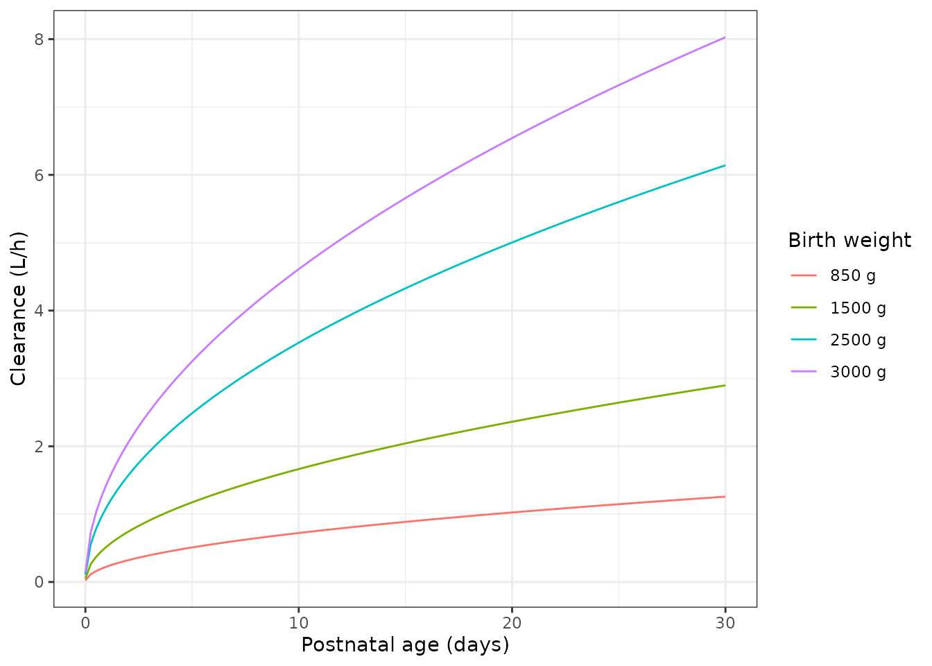
Figure 3: 1 ug/kg/h continuous infusion for 7 days
Replicates Figure 3 of Wu 2022. The Results quote three medians after
48 h of infusion: 2.1 ug/L at birth weight 850 g and postnatal age 0.5
days at the start, 1.29 ug/L at 3000 g and 0.5 days, and 0.68 ug/L at
850 g and 21 days. The deterministic comparison below uses the
typical-value (zeroRe) prediction. The stochastic medians
in the figure come from 100 virtual neonates per arm.
arms3 <- expand.grid(bw = c(0.85, 1.5, 2.5, 3.0), pna0 = c(0.5, 7, 21))
ev3 <- dplyr::bind_rows(lapply(seq_len(nrow(arms3)), function(i) {
  make_subject(
    i, arms3$bw[i], arms3$pna0[i], infusion(arms3$bw[i], 1, 168), 168,
    group = paste0("BW ", arms3$bw[i] * 1000, " g, PNA ", arms3$pna0[i], " d")
  )
}))
typ3 <- rxode2::rxSolve(mod_typ, ev3, keep = c("group", "bw", "pna0"), returnType = "data.frame")
#> ℹ omega/sigma items treated as zero: 'etalcl', 'etalvc'
#> Warning: multi-subject simulation without without 'omega'
c48 <- function(bw, pna0) {
  v <- typ3$Cc[typ3$bw == bw & typ3$pna0 == pna0 & typ3$time == 48]
  if (length(v) != 1L) stop("no unique 48 h row for BW ", bw, " PNA ", pna0)
  v
}
fig3_chk <- data.frame(
  case = c("BW 850 g, PNA 0.5 d", "BW 3000 g, PNA 0.5 d", "BW 850 g, PNA 21 d"),
  published = c(2.1, 1.29, 0.68),
  model = c(c48(0.85, 0.5), c48(3.0, 0.5), c48(0.85, 21))
) |>
  dplyr::mutate(pct_diff = 100 * (model / published - 1))
fig3_chk |>
  dplyr::rename(
    "Neonate (start of infusion)" = case, "Published median at 48 h (ug/L)" = published,
    "Model typical value at 48 h (ug/L)" = model, "% diff" = pct_diff
  ) |>
knitr::kable(digits = 2)| Neonate (start of infusion) | Published median at 48 h (ug/L) | Model typical value at 48 h (ug/L) | % diff |
|---|---|---|---|
| BW 850 g, PNA 0.5 d | 2.10 | 2.14 | 2.12 |
| BW 3000 g, PNA 0.5 d | 1.29 | 1.39 | 8.12 |
| BW 850 g, PNA 21 d | 0.68 | 0.77 | 13.27 |
# Deterministic typical-value solve. The two early-start cases sit within 8%.
# The 21-day case reads 13% high because current weight is held at birth
# weight: at 21 days the real neonate is heavier, so V1 is larger and the
# 48-h concentration is lower.
stopifnot(
  abs(fig3_chk$pct_diff[1]) < 5,
  abs(fig3_chk$pct_diff[2]) < 10,
  abs(fig3_chk$pct_diff[3]) < 20
)
rxode2::rxSetSeed(20220301)
n_per_arm <- 100
ev3_iiv <- dplyr::bind_rows(lapply(seq_len(nrow(arms3)), function(i) {
  dplyr::bind_rows(lapply(seq_len(n_per_arm), function(j) {
    make_subject(
      (i - 1) * n_per_arm + j, arms3$bw[i], arms3$pna0[i],
      infusion(arms3$bw[i], 1, 168), 168, dt = 2,
      group = paste0("PNA ", arms3$pna0[i], " d at start")
    )
  }))
}))
sim3 <- rxode2::rxSolve(mod(), ev3_iiv, keep = c("group", "bw", "pna0"), returnType = "data.frame")
med3 <- sim3 |>
  dplyr::group_by(group, bw, time) |>
  dplyr::summarise(med = median(Cc), .groups = "drop") |>
  dplyr::mutate(BW = factor(paste(bw * 1000, "g"), levels = paste(c(850, 1500, 2500, 3000), "g")))
ggplot(med3, aes(time, med, colour = BW)) +
  geom_line() +
  facet_wrap(~group) +
  labs(
    x = "Time since start of infusion (h)", y = "Median fentanyl concentration (ug/L)",
    colour = "Birth weight",
    caption = "Replicates Figure 3 of Wu 2022 (current weight held at birth weight)."
  ) +
  theme_bw()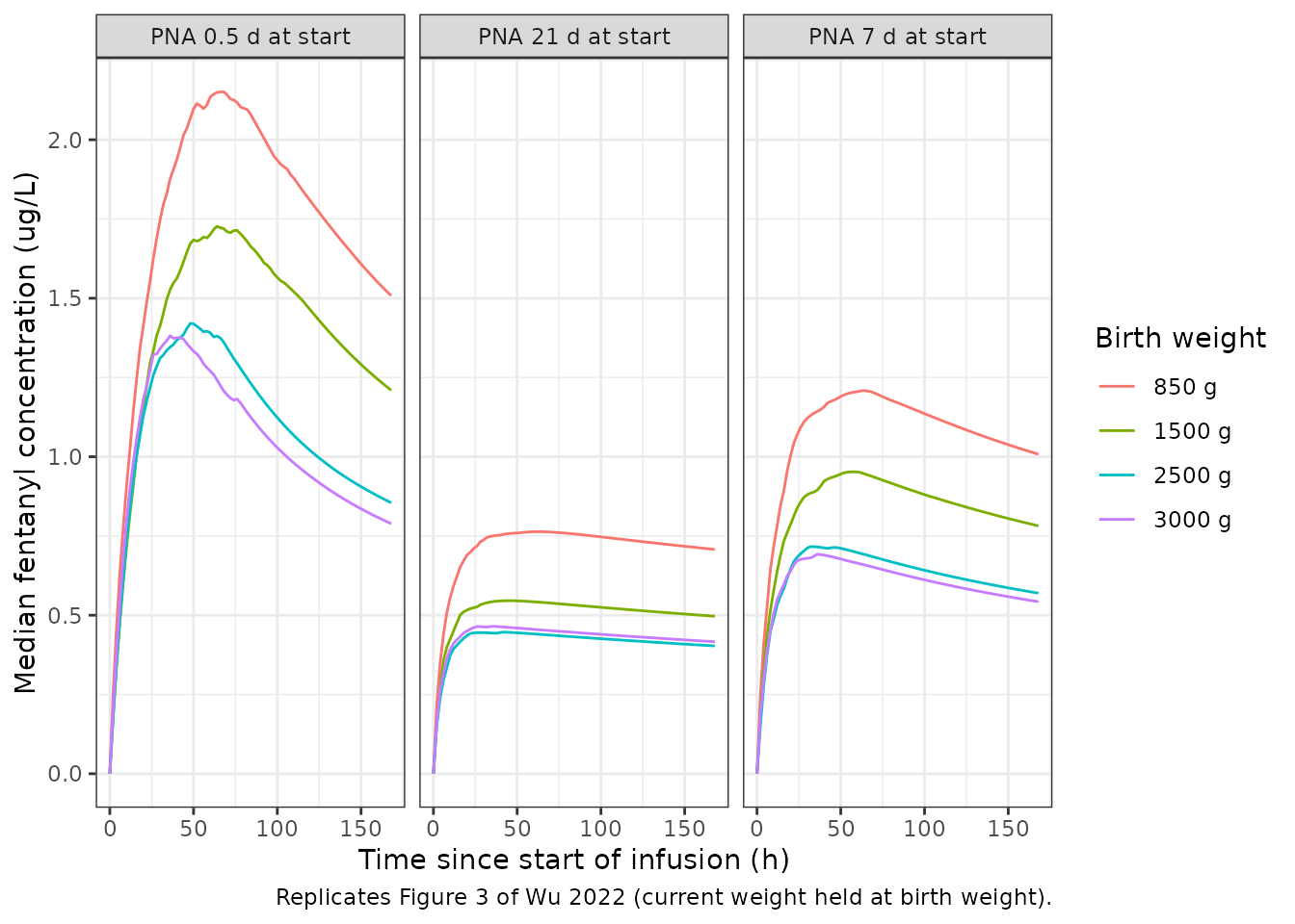
As in the paper, concentrations rise for 1-2 days before they peak. They fall as birth weight rises and, within a birth weight, as postnatal age at the start of treatment rises. The later decline the paper shows comes partly from current weight increasing over the week, which this simulation leaves out.
Figure 5: intermittent boluses with and without a loading dose
Replicates Figure 5 of Wu 2022, typical-value profiles at postnatal age 0.5 days. (A) 2 ug/kg every 4 h for 2 days. (B) A 5 ug/kg loading dose over 3 min, then 2 ug/kg every 4 h. The Results state that the loading dose reaches “around 0.75-1.2 ug/L” immediately at 850 g and “around 0.5 ug/L” in larger neonates.
q4h <- seq(0, 44, by = 4)
arms5 <- expand.grid(bw = c(0.85, 1.5, 2.5, 3.0), regimen = c("A: 2 ug/kg q4h", "B: 5 ug/kg load + 2 ug/kg q4h"), stringsAsFactors = FALSE)
ev5 <- dplyr::bind_rows(lapply(seq_len(nrow(arms5)), function(i) {
  bw <- arms5$bw[i]
  d <- if (startsWith(arms5$regimen[i], "A")) {
    boluses(bw, 2, q4h)
  } else {
    dplyr::bind_rows(boluses(bw, 5, 0), boluses(bw, 2, q4h[-1]))
  }
  make_subject(i, bw, 0.5, d, 48, dt = 0.05, group = arms5$regimen[i])
}))
typ5 <- rxode2::rxSolve(mod_typ, ev5, keep = c("group", "bw"), returnType = "data.frame") |>
  dplyr::mutate(BW = factor(paste(bw * 1000, "g"), levels = paste(c(850, 1500, 2500, 3000), "g")))
#> ℹ omega/sigma items treated as zero: 'etalcl', 'etalvc'
#> Warning: multi-subject simulation without without 'omega'
ggplot(typ5, aes(time, Cc, colour = BW)) +
  geom_line() +
  facet_wrap(~group) +
  labs(x = "Time (h)", y = "Typical fentanyl concentration (ug/L)", colour = "Birth weight") +
  theme_bw()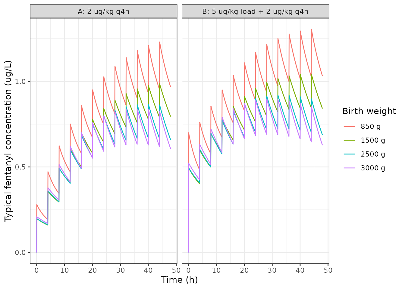
load_peak <- typ5 |>
  dplyr::filter(startsWith(group, "B"), time <= 4) |>
  dplyr::group_by(BW) |>
  dplyr::summarise(peak_after_load = max(Cc), .groups = "drop")
knitr::kable(load_peak |> dplyr::rename("Birth weight" = BW, "Peak after loading dose (ug/L)" = peak_after_load), digits = 2)| Birth weight | Peak after loading dose (ug/L) |
|---|---|
| 850 g | 0.70 |
| 1500 g | 0.50 |
| 2500 g | 0.50 |
| 3000 g | 0.52 |
The model gives about 0.7 ug/L at 850 g and about 0.5 ug/L at 1500-3000 g. That matches the paper’s “around 0.5 ug/L” for larger neonates and falls just below the 0.75 ug/L lower end quoted for 850 g. This is a typical-value prediction at postnatal age 0.5 days. The paper’s statement covers several postnatal ages and is read from a figure of medians.
PKNCA: the proposed regimen (Table 3) vs the published AUC envelope
Wu 2022 Table 3 proposes 0.5/0.7/0.9 ug/kg/h below 1500 g and 0.7/0.9/1.2 ug/kg/h at or above 1500 g, for postnatal ages of 1-2, 3-6 and >= 7 days at the start of treatment. For this regimen the authors report (Results 3.2.1 and ESM Fig. S5) daily AUCs of 9-16 ug*h/L on day 1, 12-26 on day 4 and 11-24 on day 7, and concentrations of 0.6-1.2 ug/L after 24 h. The simulation below gives each typical neonate a constant rate chosen from its postnatal age at the start. It excludes birth weight >= 2500 g with postnatal age > 7 days, as the paper does. PKNCA computes the three daily AUCs per neonate.
rate_t3 <- function(bw, pna0) {
  band <- 1L + (pna0 >= 3) + (pna0 >= 7)
  if (bw < 1.5) c(0.5, 0.7, 0.9)[band] else c(0.7, 0.9, 1.2)[band]
}
arms_t3 <- expand.grid(bw = c(0.85, 1.5, 2.5, 3.0), pna0 = c(1, 3, 7))
arms_t3$rate <- mapply(rate_t3, arms_t3$bw, arms_t3$pna0)
arms_t3$treatment <- paste0("BW ", arms_t3$bw * 1000, " g, PNA ", arms_t3$pna0, " d, ", arms_t3$rate, " ug/kg/h")
ev_t3 <- dplyr::bind_rows(lapply(seq_len(nrow(arms_t3)), function(i) {
  make_subject(i, arms_t3$bw[i], arms_t3$pna0[i], infusion(arms_t3$bw[i], arms_t3$rate[i], 168), 168,
    dt = 0.25, group = arms_t3$treatment[i]
  )
}))
typ_t3 <- rxode2::rxSolve(mod_typ, ev_t3, keep = c("group"), returnType = "data.frame") |>
  dplyr::rename(treatment = group)
#> ℹ omega/sigma items treated as zero: 'etalcl', 'etalvc'
#> Warning: multi-subject simulation without without 'omega'

conc_df <- typ_t3 |>
  dplyr::filter(!is.na(Cc)) |>
  dplyr::select(id, treatment, time, Cc)
dose_df <- ev_t3 |>
  dplyr::filter(evid == 1) |>
  dplyr::transmute(id, treatment = group, time, amt)
o_conc <- PKNCA::PKNCAconc(conc_df, Cc ~ time | treatment + id)
o_dose <- PKNCA::PKNCAdose(dose_df, amt ~ time | treatment + id)
intervals <- data.frame(
  start = c(0, 72, 144), end = c(24, 96, 168),
  auclast = TRUE
)
nca_t3 <- PKNCA::pk.nca(PKNCA::PKNCAdata(o_conc, o_dose, intervals = intervals))
auc_t3 <- as.data.frame(nca_t3$result) |>
  dplyr::filter(PPTESTCD == "auclast") |>
  dplyr::mutate(day = c(`0` = "Day 1", `72` = "Day 4", `144` = "Day 7")[as.character(start)])
stopifnot(nrow(auc_t3) == 3L * nrow(arms_t3))

c24_t3 <- typ_t3 |> dplyr::filter(time == 24)
stopifnot(nrow(c24_t3) == nrow(arms_t3))

envelope <- data.frame(
  quantity = c("Day 1", "Day 4", "Day 7", "Concentration at 24 h (ug/L)"),
  published_low = c(9, 12, 11, 0.6),
  published_high = c(16, 26, 24, 1.2)
)
sim_range <- auc_t3 |>
  dplyr::group_by(quantity = day) |>
  dplyr::summarise(sim_low = min(PPORRES), sim_high = max(PPORRES), .groups = "drop") |>
  dplyr::bind_rows(data.frame(
    quantity = "Concentration at 24 h (ug/L)",
    sim_low = min(c24_t3$Cc), sim_high = max(c24_t3$Cc)
  ))
env_tab <- dplyr::left_join(envelope, sim_range, by = "quantity") |>
  dplyr::mutate(quantity = ifelse(startsWith(quantity, "Day"), paste(quantity, "AUC (ug*h/L)"), quantity))
env_tab |>
  dplyr::rename(
    "Quantity" = quantity, "Published low" = published_low, "Published high" = published_high,
    "Simulated low" = sim_low, "Simulated high" = sim_high
  ) |>
knitr::kable(digits = 2)| Quantity | Published low | Published high | Simulated low | Simulated high |
|---|---|---|---|---|
| Day 1 AUC (ug*h/L) | 9.0 | 16.0 | 11.42 | 16.85 |
| Day 4 AUC (ug*h/L) | 12.0 | 26.0 | 17.37 | 25.89 |
| Day 7 AUC (ug*h/L) | 11.0 | 24.0 | 12.97 | 22.67 |
| Concentration at 24 h (ug/L) | 0.6 | 1.2 | 0.78 | 1.04 |
auc_t3 |>
  dplyr::select(treatment, day, PPORRES) |>
  tidyr::pivot_wider(names_from = day, values_from = PPORRES) |>
  dplyr::left_join(c24_t3 |> dplyr::select(treatment, Cc), by = "treatment") |>
  dplyr::rename(
    "Typical neonate and Table 3 rate" = treatment,
    "Day 1 AUC (ug*h/L)" = `Day 1`, "Day 4 AUC (ug*h/L)" = `Day 4`,
    "Day 7 AUC (ug*h/L)" = `Day 7`, "C at 24 h (ug/L)" = Cc
  ) |>
knitr::kable(digits = 2)| Typical neonate and Table 3 rate | Day 1 AUC (ug*h/L) | Day 4 AUC (ug*h/L) | Day 7 AUC (ug*h/L) | C at 24 h (ug/L) |
|---|---|---|---|---|
| BW 1500 g, PNA 1 d, 0.7 ug/kg/h | 13.22 | 24.45 | 18.29 | 0.92 |
| BW 1500 g, PNA 3 d, 0.9 ug/kg/h | 14.87 | 25.29 | 20.56 | 0.98 |
| BW 1500 g, PNA 7 d, 1.2 ug/kg/h | 16.85 | 25.89 | 22.67 | 1.04 |
| BW 2500 g, PNA 1 d, 0.7 ug/kg/h | 12.81 | 19.07 | 14.20 | 0.85 |
| BW 2500 g, PNA 3 d, 0.9 ug/kg/h | 13.95 | 19.74 | 16.04 | 0.87 |
| BW 2500 g, PNA 7 d, 1.2 ug/kg/h | 15.28 | 20.26 | 17.75 | 0.89 |
| BW 3000 g, PNA 1 d, 0.7 ug/kg/h | 12.97 | 17.37 | 12.97 | 0.84 |
| BW 3000 g, PNA 3 d, 0.9 ug/kg/h | 13.86 | 18.04 | 14.68 | 0.84 |
| BW 3000 g, PNA 7 d, 1.2 ug/kg/h | 14.90 | 18.56 | 16.27 | 0.84 |
| BW 850 g, PNA 1 d, 0.5 ug/kg/h | 11.42 | 22.64 | 17.22 | 0.78 |
| BW 850 g, PNA 3 d, 0.7 ug/kg/h | 14.08 | 25.63 | 21.01 | 0.92 |
| BW 850 g, PNA 7 d, 0.9 ug/kg/h | 15.52 | 25.36 | 22.27 | 0.96 |
# Deterministic typical-value solve. Day 4, day 7 and the 24 h concentration
# fall inside the published envelopes. The day-1 maximum (16.8 ug*h/L at
# 1500 g, PNA 7 d, 1.2 ug/kg/h) is 5% above the published 16. The gate allows
# 10% on the envelope edges, which still fails on a mis-transcribed clearance,
# volume or dose unit, since any of those moves the whole range by tens of
# percent.
rng <- function(q) unlist(env_tab[env_tab$quantity == q, c("sim_low", "sim_high")])
stopifnot(
  all(rng("Concentration at 24 h (ug/L)") >= 0.6 & rng("Concentration at 24 h (ug/L)") <= 1.2),
  all(rng("Day 4 AUC (ug*h/L)") >= 12 & rng("Day 4 AUC (ug*h/L)") <= 26),
  all(rng("Day 7 AUC (ug*h/L)") >= 11 & rng("Day 7 AUC (ug*h/L)") <= 24),
  all(rng("Day 1 AUC (ug*h/L)") >= 9 * 0.9 & rng("Day 1 AUC (ug*h/L)") <= 16 * 1.1)
)
PKNCA mass balance: AUC(0-inf) x CL = dose
With postnatal age held constant (so clearance is time-invariant), a
single 2 ug/kg bolus must give AUCinf * CL = dose for every
typical neonate. This checks the ODE system and the dose, volume and
clearance units.
arms_mb <- expand.grid(bw = c(0.5, 0.85, 1.5, 3.0), pna0 = c(1, 7))
ev_mb <- dplyr::bind_rows(lapply(seq_len(nrow(arms_mb)), function(i) {
  bw <- arms_mb$bw[i]
  obs_t <- sort(unique(c(seq(0, 1, by = 0.05), seq(1, 24, by = 0.5), seq(24, 1500, by = 4))))
  d <- dplyr::bind_rows(
    data.frame(id = i, time = 0, evid = 1L, amt = 2 * bw, rate = 2 * bw / 0.05, cmt = "central"),
    data.frame(id = i, time = obs_t, evid = 0L, amt = 0, rate = 0, cmt = "central")
  ) |> dplyr::arrange(time, dplyr::desc(evid))
  d$WT_BIRTH <- bw
  d$WT <- bw
  d$PNA <- arms_mb$pna0[i] / 30.4375 # held constant
  d$STUDY_DINO <- 1L
  d$treatment <- paste0("BW ", bw * 1000, " g, PNA ", arms_mb$pna0[i], " d")
  d
}))
typ_mb <- rxode2::rxSolve(mod_typ, ev_mb, keep = "treatment", returnType = "data.frame")
#> ℹ omega/sigma items treated as zero: 'etalcl', 'etalvc'
#> Warning: multi-subject simulation without without 'omega'
nca_mb <- PKNCA::pk.nca(PKNCA::PKNCAdata(
  PKNCA::PKNCAconc(typ_mb |> dplyr::filter(!is.na(Cc)) |> dplyr::select(id, treatment, time, Cc), Cc ~ time | treatment + id),
  PKNCA::PKNCAdose(ev_mb |> dplyr::filter(evid == 1) |> dplyr::select(id, treatment, time, amt), amt ~ time | treatment + id),
  intervals = data.frame(start = 0, end = Inf, aucinf.obs = TRUE)
))
mb <- as.data.frame(nca_mb$result) |>
  dplyr::filter(PPTESTCD == "aucinf.obs") |>
  dplyr::left_join(typ_mb |> dplyr::distinct(treatment, cl), by = "treatment") |>
  dplyr::left_join(ev_mb |> dplyr::filter(evid == 1) |> dplyr::distinct(treatment, amt), by = "treatment") |>
  dplyr::mutate(ratio = PPORRES * cl / amt)
mb |>
  dplyr::select(treatment, PPORRES, cl, amt, ratio) |>
  dplyr::rename(
    "Typical neonate" = treatment, "AUCinf (ug*h/L)" = PPORRES,
    "CL (L/h)" = cl, "Dose (ug)" = amt, "AUCinf x CL / dose" = ratio
  ) |>
knitr::kable(digits = 3)| Typical neonate | AUCinf (ug*h/L) | CL (L/h) | Dose (ug) | AUCinf x CL / dose |
|---|---|---|---|---|
| BW 1500 g, PNA 1 d | 5.740 | 0.523 | 3.0 | 1 |
| BW 1500 g, PNA 7 d | 2.158 | 1.390 | 3.0 | 1 |
| BW 3000 g, PNA 1 d | 4.144 | 1.448 | 6.0 | 1 |
| BW 3000 g, PNA 7 d | 1.558 | 3.852 | 6.0 | 1 |
| BW 500 g, PNA 1 d | 9.621 | 0.104 | 1.0 | 1 |
| BW 500 g, PNA 7 d | 3.618 | 0.277 | 1.0 | 1 |
| BW 850 g, PNA 1 d | 7.497 | 0.227 | 1.7 | 1 |
| BW 850 g, PNA 7 d | 2.818 | 0.603 | 1.7 | 1 |
Assumptions and deviations
- Eq. 2 exponents. The article’s Eq. 2 prints 1.57 and 0.502. Table 2 prints 1.47 and 0.505. Table 2 is used because it reproduces all five published clearance fold-changes, and the ESM initial value of the birth-weight exponent is also 1.47 (see “Printed Eq. 2 exponents vs Table 2”).
-
IIV scale. The printed IIV percentages are read as
100*omega(see “IIV scale”). The exact-CV reading would give omega^2 of 0.180 and 0.189 instead of 0.197 and 0.208. -
Proportional residual error. Table 2 labels the
proportional rows “(%)” but prints 0.23 and 0.361. With
$SIGMA 1 FIXandW = SQRT(ADD**2 + (PRO*IPRED)**2)in the ESM$ERRORblock, these are fractional SDs (23% and 36.1%). -
Dataset indicator. The residual magnitudes depend
on the dataset (ESM column
ASY), encoded asSTUDY_DINO(1 = DINO dataset 2, 0 = Helsinki dataset 1). The simulations here useSTUDY_DINO = 1. Only simulated observations with residual error depend on it;Ccdoes not. - Current body weight. The authors projected current weight from birth weight with the Anchieta growth curves. Those curves are not given numerically, so these simulations hold current weight at birth weight. This mainly affects the 21-day arm of Figure 3.
- Table 3 rate. The simulations hold each neonate’s Table 3 rate at the value for its postnatal age at the start of treatment. The paper does not say whether its Fig. S5 simulation stepped the rate up as postnatal age crossed a band boundary.
-
Postnatal-age units. The source uses days. The
canonical
PNAcolumn is in months, and the model converts it back (PNA * 30.4375).