FXI antisense oligonucleotides: IONIS-FXIRX and FXI-LICA (Willmann 2021) • nlmixr2lib

Model and source

Citation: Willmann S, Marostica E, Snelder N, Solms A, Jensen M, Lobmeyer M, Lensing AWA, Bethune C, Morgan E, Yu RZ, Wang Y, Jung SW, Geary R, Bhanot S. PK/PD modeling of FXI antisense oligonucleotides to bridge the dose-FXI activity relation from healthy volunteers to end-stage renal disease patients. CPT Pharmacometrics Syst Pharmacol. 2021;10(8):890-901.
DOI: https://doi.org/10.1002/psp4.12663
Packaged models:
- Willmann_2021_ionisFxirx – IONIS-FXIRX (BAY2306001) PK/PD in healthy volunteers (study ASO-CS1) and patients with end-stage renal disease on hemodialysis (study ASO-CS4).
- Willmann_2021_fxiLica – FXI-LICA (BAY2976217, formerly ION-957943) PK/PD in healthy volunteers (study LICA-CS1), with the ESRD covariate effects borrowed from IONIS-FXIRX for the paper’s FXI-LICA-in-ESRD simulation scenario.

The two compounds share the same structural PK/PD backbone (Figure 2 of the paper) but were fitted with separate PK parameters (Tables S2 and S3) and share a jointly-fitted indirect-response arm on FXI activity (Table S4). Each drug is therefore packaged as a distinct model file, and this single vignette walks the paper’s bridging analysis by exercising each modellib() entry at the appropriate step.

Structural model

The pharmacokinetic model is two-compartment with parallel first-order and zero-order subcutaneous absorption:

Fraction $F_1$ of the dose enters depot and is absorbed first-order with rate $k_a$ into central.
Fraction $1 - F_1$ enters central directly as a zero-order input over duration $D_2$ .
Central and peripheral compartments (volumes $V_2$ and $V_3$ , intercompartmental clearance $Q$ ) with first-order elimination from central (clearance $CL$ ).

The pharmacodynamic model is an indirect-response turnover model for FXI activity with a sigmoid-Imax inhibition of the zero-order synthesis rate $K_{in} = \text{Baseline} \cdot k_{out}$ :

$\frac{d \text{FXIact}}{dt} = K_{in} \cdot \left(1 - \frac{I_{max} \cdot C_e^{\gamma}}{IC_{50}^{\gamma} + C_e^{\gamma}}\right) - k_{out} \cdot \text{FXIact}$

with $I_{max}$ fixed to 1 and Hill exponent $\gamma$ shared across compounds and studies. The inhibitory driver $C_e$ is the concentration in an effect compartment linked to plasma via first-order equilibration ( $k_{eo}$ ):

$\frac{d C_e}{dt} = k_{eo} \cdot \left( k_{eo\_pat}^{\text{ESRD}} \cdot C_c - C_e \right)$

The paper’s keoPAT factor scales the effect-site driving concentration in ESRD patients (keoPAT = 0.329 -> $C_{e,ss}$ in ESRD is $$1/3 of the HV value at the same $C_c$ ; note the paper’s Discussion phrases this as “a factor of approximately one-third on the effect site concentration”).

Dosing convention

Because the PK has parallel absorption arms, each administration must be encoded as two dose event rows: one targeting cmt = "depot" (first-order, fraction $F_1$ ) and one targeting cmt = "central" (zero-order, fraction $1 - F_1$ , duration $D_2$ ). The zero-order row must set rate = -2 so rxode2 uses the model-defined dur(central) <- d1 value; otherwise the zero-order component collapses to an instantaneous bolus.

Doses are entered in mg; simulated $C_c$ is returned in ng/mL (the units the paper reports).

Population

Study cohorts (Willmann 2021 Supplementary Information Table S1):

Study	Drug	Phase	Cohort	n active	n placebo	Weight (mean SD)	Age (mean SD)
ASO-CS1	IONIS-FXIRX	1	Healthy volunteers	66	22	72.7 (10.5) kg	45.4 (11.9) years
ASO-CS4	IONIS-FXIRX	2	ESRD on hemodialysis	36	13	87.8 (22.7) kg	59.2 (12.9) years
LICA-CS1	FXI-LICA	1	Healthy volunteers (FIH)	48	18	77.5 (13.2) kg	50.8 (11.5) years

Weight in ASO-CS4 spans 48.5-164 kg (Methods, “PK/PD simulations for FXI-LICA in patients with ESRD”). Race and ethnicity are not reported in the primary publication.

Per-drug demographic metadata is available via readModelDb(name)$population.

Source trace

The per-parameter origin is recorded as an in-file comment next to each ini() entry in the two model files under inst/modeldb/specificDrugs/. The table below consolidates them for review.

Equation / parameter	Value	Source location
Structural PK: 2-cmt, parallel first-order + zero-order absorption, first-order elimination	n/a	Willmann 2021 Methods; Figure 2
Structural PD: indirect response with sigmoid Imax on Kin, effect-site driver	n/a	Willmann 2021 Methods; Figure 2
IONIS-FXIRX PK (Table S2)
`lcl` (CL, HV)	log(3.12)	Willmann 2021 Table S2
`lvc` (V2 at 70 kg)	log(9.55)	Willmann 2021 Table S2
`lq` (Q)	log(0.202)	Willmann 2021 Table S2
`lvp` (V3, HV)	log(164)	Willmann 2021 Table S2
`lka` (ka)	log(0.191)	Willmann 2021 Table S2
`ld1` (D2)	log(4.88)	Willmann 2021 Table S2
`logitfdepot` (Logit F1)	qlogis(0.688) = 0.790	Willmann 2021 Table S2
`e_esrd_cl` (ESRD on CL)	0.530 fixed	Willmann 2021 Table S2
`e_esrd_vp` (ESRD on V3)	0.379 fixed	Willmann 2021 Table S2
`e_wt_vc` (BWT on V2)	0.967 fixed	Willmann 2021 Table S2
FXI-LICA PK (Table S3)
`lcl` (CL)	log(12.8)	Willmann 2021 Table S3
`lvc` (V2)	log(48.9)	Willmann 2021 Table S3
`lq` (Q)	log(1.82)	Willmann 2021 Table S3
`lvp` (V3)	log(924)	Willmann 2021 Table S3
`lka` (ka)	log(0.864)	Willmann 2021 Table S3
`ld1` (D2)	log(9.38)	Willmann 2021 Table S3
`logitfdepot` (Logit F1)	qlogis(0.620) = 0.490	Willmann 2021 Table S3
OMEGA BLOCK (CL, V2, Q)	0.146 / 0.172 / 0.312 / 0.127 / 0.189 / 0.234	Willmann 2021 Table S3
Joint PK/PD (Table S4)
`imax` (Imax)	1.00 fixed	Willmann 2021 Table S4
`lic50` (IC50, IONIS-FXIRX)	log(167)	Willmann 2021 Table S4
`lic50` (IC50, FXI-LICA)	log(2.59)	Willmann 2021 Table S4
`lrbase` (Baseline)	log(0.994)	Willmann 2021 Table S4
`lkout` (kout)	log(0.00435)	Willmann 2021 Table S4
`lhill` (gamma)	log(1.50)	Willmann 2021 Table S4
`lke0` (keo)	log(0.00115)	Willmann 2021 Table S4
`le_esrd_effect` (log keoPAT)	log(0.329) fixed	Willmann 2021 Table S4
Residual PK (Cc) ASO-CS1	0.229 prop	Willmann 2021 Table S2
Residual PK (Cc) ASO-CS4	0.290 prop	Willmann 2021 Table S2
Residual PK (Cc) LICA-CS1	0.259 prop	Willmann 2021 Table S3
Residual PD (FXIact) ASO-CS1	0.0851 prop	Willmann 2021 Table S4
Residual PD (FXIact) ASO-CS4	0.172 prop	Willmann 2021 Table S4
Residual PD (FXIact) LICA-CS1	0.101 prop	Willmann 2021 Table S4

Virtual cohort

The published individual-level data are not publicly available. The figures below use deterministic typical-value simulations plus small stochastic cohorts (uniform body weight per the ESRD range for FXI-LICA-in-ESRD scenarios, and normal $N(72.7, 10.5)$ weight for HV cohorts, capped to a reasonable range). Cohort sizes are kept below 200 per arm; larger cohorts add no validation value and materially increase render time.

set.seed(20210801L)

# Build a two-row dose event pattern for the mixed absorption model.
# Doses are entered in mg. The zero-order row uses rate = -2 so
# rxode2 picks up the model-defined dur(central) <- d1. `subjects` is
# a data.frame with columns id, wt, esrd, dose_mg (one row per
# subject).
make_events <- function(subjects, dose_times, obs_times) {
  # Dose rows: two rows per (subject, dose_time).
  n_sub <- nrow(subjects)
  n_dose <- length(dose_times)
  n_obs <- length(obs_times)
  doses <- data.frame(
    id = rep(subjects$id, each = n_dose * 2L),
    time = rep(rep(dose_times, each = 2L), times = n_sub),
    evid = 1L,
    amt = rep(subjects$dose_mg, each = n_dose * 2L),
    cmt = rep(c("depot", "central"), times = n_sub * n_dose),
    rate = rep(c(0, -2), times = n_sub * n_dose),
    dur = 0,
    dvid = NA_real_,
    WT = rep(subjects$wt, each = n_dose * 2L),
    RRT_HEMODIAL_STATUS = rep(subjects$esrd, each = n_dose * 2L),
    dose_mg = rep(subjects$dose_mg, each = n_dose * 2L),
    stringsAsFactors = FALSE
  )
  # Observation rows: one per (subject, obs_time). The model declares
  # TWO outputs with residual error (Cc and FXIact); rxode2 therefore
  # needs a `dvid` column on observation rows to disambiguate which
  # output the row targets. `dvid = 1L` selects the first residual
  # declared (Cc); rxode2 still returns both Cc and FXIact as columns
  # in the solved output, so this only tags the "primary" DV for the
  # observation record.
  obs <- data.frame(
    id = rep(subjects$id, each = n_obs),
    time = rep(obs_times, times = n_sub),
    evid = 0L,
    amt = 0,
    cmt = NA_character_,
    rate = 0,
    dur = 0,
    dvid = 1L,
    WT = rep(subjects$wt, each = n_obs),
    RRT_HEMODIAL_STATUS = rep(subjects$esrd, each = n_obs),
    dose_mg = rep(subjects$dose_mg, each = n_obs),
    stringsAsFactors = FALSE
  )
  dplyr::bind_rows(doses, obs) |>
    dplyr::arrange(id, time, dplyr::desc(evid))
}

Simulation: IONIS-FXIRX in healthy volunteers

Study ASO-CS1 gave IONIS-FXIRX as single and multiple SC doses at 50-300 mg. Reproduce a typical-value single-dose 300 mg profile in an HV (WT = 70 kg, ESRD = 0).

mod_ionis <- nlmixr2lib::readModelDb("Willmann_2021_ionisFxirx")
mod_ionis_typ <- rxode2::zeroRe(mod_ionis)
#> ℹ parameter labels from comments will be replaced by 'label()'

# Deterministic typical-value single-dose 300 mg IONIS-FXIRX in HV.
subjects_ionis_hv <- data.frame(
  id = 1L, wt = 70, esrd = 0, dose_mg = 300
)
ev_ionis_hv <- make_events(
  subjects_ionis_hv,
  dose_times = 0,
  obs_times = c(0, 0.5, 1, 1.5, 2, 3, 4, 6, 8, 12, 24,
                48, 72, 96, 168, 336, 504, 672)
)

sim_ionis_hv <- rxode2::rxSolve(
  mod_ionis_typ, events = ev_ionis_hv,
  keep = c("WT", "RRT_HEMODIAL_STATUS")
) |> as.data.frame()
#> ℹ omega/sigma items treated as zero: 'etalcl', 'etalvc', 'etalq', 'etalvp', 'etalka', 'etalogitfdepot', 'etalrbase', 'etalic50', 'etalkout', 'etalke0'

ggplot(sim_ionis_hv, aes(time / 24, Cc)) +
  geom_line(colour = "steelblue", linewidth = 0.8) +
  scale_y_log10() +
  labs(x = "Time (days)", y = "IONIS-FXIRX plasma Cc (ng/mL)",
       title = "Typical-value single 300 mg SC dose in an HV") +
  theme_bw()
#> Warning in scale_y_log10(): log-10 transformation introduced infinite values.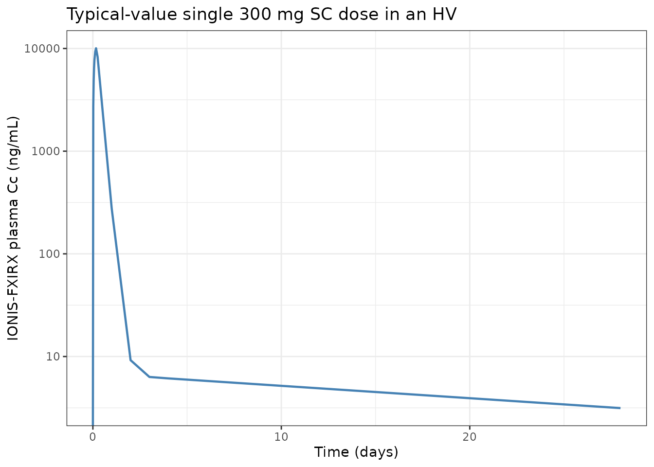

Simulation: IONIS-FXIRX in ESRD patients

Study ASO-CS4 (ESRD, once every 28 days for up to 12 weeks) is the setting where the ESRD covariates (CL x 0.47, V3 x 0.62, effect-site driving concentration x 0.329) are activated. Repeat a typical-value 300 mg once-monthly regimen for 4 doses.

# Multiple-dose 300 mg every 28 days, ESRD = 1.
dose_times_q28 <- 24 * 28 * (0:3)   # 4 doses at 0, 28, 56, 84 days (in h)
obs_times_q28 <- sort(unique(c(0, dose_times_q28, seq(0, 24 * 200, by = 24))))

subjects_ionis_esrd <- data.frame(
  id = 1L, wt = 88, esrd = 1, dose_mg = 300
)
ev_ionis_esrd <- make_events(
  subjects_ionis_esrd,
  dose_times = dose_times_q28,
  obs_times = obs_times_q28
)

sim_ionis_esrd <- rxode2::rxSolve(
  mod_ionis_typ, events = ev_ionis_esrd,
  keep = c("WT", "RRT_HEMODIAL_STATUS")
) |> as.data.frame()
#> ℹ omega/sigma items treated as zero: 'etalcl', 'etalvc', 'etalq', 'etalvp', 'etalka', 'etalogitfdepot', 'etalrbase', 'etalic50', 'etalkout', 'etalke0'

ggplot(sim_ionis_esrd, aes(time / 24, FXIact)) +
  geom_line(colour = "darkred", linewidth = 0.8) +
  geom_hline(yintercept = 0.2, linetype = 2, colour = "gray30") +
  labs(x = "Time (days)", y = "FXI activity (U/mL)",
       title = "IONIS-FXIRX 300 mg every 28 days in ESRD (typical value)",
       subtitle = "Dashed line: 0.20 U/mL, the TKA study 300 mg cohort observed mean") +
  theme_bw()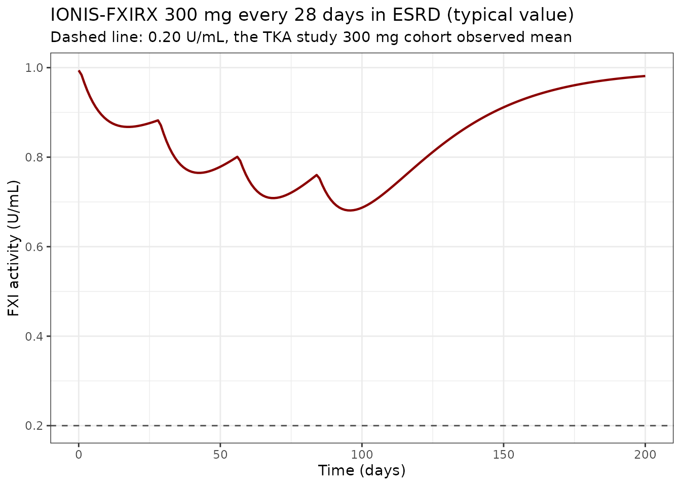

The 300 mg once-monthly IONIS-FXIRX regimen reaches steady-state FXI activity of $$0.2 U/mL in ESRD, consistent with the mean 0.20 U/mL observed in the 300 mg cohort of the IONIS-FXIRX TKA study (Willmann 2021 Discussion citing the phase II TKA study).

Simulation: FXI-LICA in healthy volunteers (LICA-CS1)

Study LICA-CS1 dose ranges: 40-120 mg single SC doses; 10-30 mg weekly x 6 or 80 mg every 4 weeks x 4. Reproduce the 80 mg every-4-weeks multiple-dose FXI-LICA HV profile.

mod_lica <- nlmixr2lib::readModelDb("Willmann_2021_fxiLica")
mod_lica_typ <- rxode2::zeroRe(mod_lica)
#> ℹ parameter labels from comments will be replaced by 'label()'

dose_times_q4w <- 24 * 28 * (0:3)   # 4 doses at 0, 28, 56, 84 days
obs_times_q4w <- sort(unique(c(0, dose_times_q4w, seq(0, 24 * 200, by = 12))))

subjects_lica_hv <- data.frame(
  id = 1L, wt = 78, esrd = 0, dose_mg = 80
)
ev_lica_hv <- make_events(
  subjects_lica_hv,
  dose_times = dose_times_q4w,
  obs_times = obs_times_q4w
)

sim_lica_hv <- rxode2::rxSolve(
  mod_lica_typ, events = ev_lica_hv,
  keep = c("WT", "RRT_HEMODIAL_STATUS")
) |> as.data.frame()
#> ℹ omega/sigma items treated as zero: 'etalcl', 'etalvc', 'etalq', 'etalvp', 'etalka', 'etalrbase', 'etalic50', 'etalkout', 'etalke0'

ggplot(sim_lica_hv, aes(time / 24, FXIact)) +
  geom_line(colour = "purple4", linewidth = 0.8) +
  labs(x = "Time (days)", y = "FXI activity (U/mL)",
       title = "FXI-LICA 80 mg every 28 days in HV (typical value)") +
  theme_bw()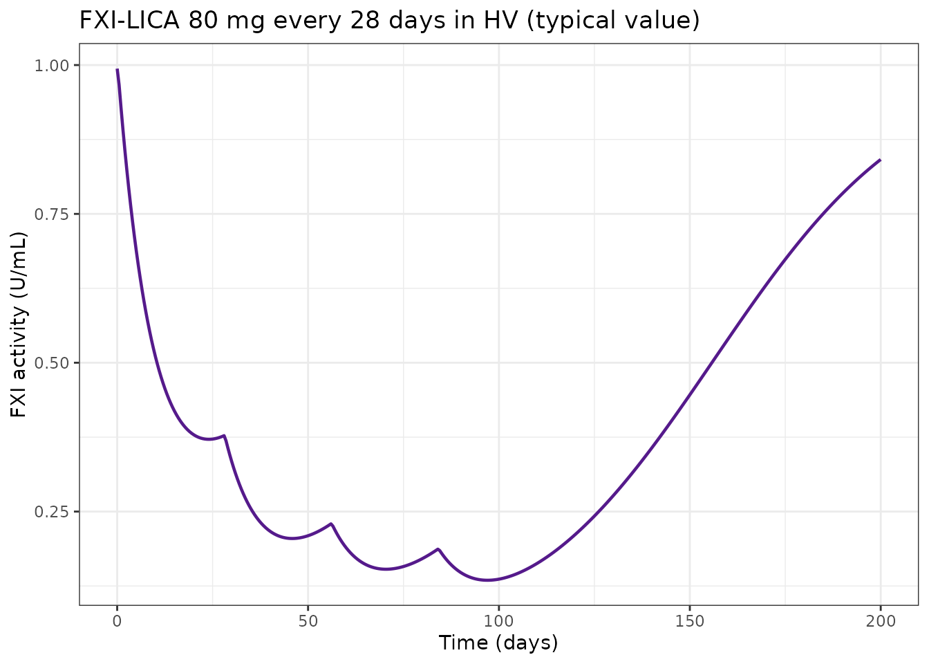

Simulation: FXI-LICA in ESRD (borrowed IONIS-FXIRX ESRD effects)

Figures 3a and 4 of Willmann 2021 predict FXI activity at steady-state for FXI-LICA once-monthly in ESRD at 40, 80, and 120 mg. Reproduce the paper’s virtual ESRD cohort (n = 100 per dose, uniform WT $[48.5, 164]$ kg per Methods) and compute the average FXI activity over a single dosing interval at steady-state.

n_per_arm <- 100L
dose_levels_mg <- c(40, 80, 120)

# Uniform weight distribution per Methods; steady-state reached
# after 4-5 doses per Results, so simulate 6 doses q28d and take
# the average FXI activity over the last dosing interval.
n_doses <- 6L
dose_times_ss <- 24 * 28 * (0:(n_doses - 1L))
obs_grid <- seq(0, 24 * 28 * n_doses, by = 12)

# Build the pooled subjects data.frame across the 3 dose arms:
# one row per subject with (id, wt, esrd, dose_mg).
build_esrd_subjects <- function() {
  do.call(rbind, lapply(seq_along(dose_levels_mg), function(k) {
    d <- dose_levels_mg[k]
    start_id <- 1000L * k
    data.frame(
      id = start_id + seq_len(n_per_arm) - 1L,
      wt = runif(n_per_arm, min = 48.5, max = 164),
      esrd = 1,
      dose_mg = d
    )
  }))
}
subjects_lica_esrd <- build_esrd_subjects()

ev_lica_esrd <- make_events(
  subjects_lica_esrd,
  dose_times = dose_times_ss,
  obs_times = obs_grid
)

sim_lica_esrd <- rxode2::rxSolve(
  mod_lica, events = ev_lica_esrd,
  keep = c("WT", "RRT_HEMODIAL_STATUS", "dose_mg")
) |> as.data.frame()
#> ℹ parameter labels from comments will be replaced by 'label()'

# Average FXI activity over the last dosing interval per subject.
last_interval_start <- 24 * 28 * (n_doses - 1L)
last_interval_end   <- 24 * 28 * n_doses
ss_avg <- sim_lica_esrd |>
  dplyr::filter(time >= last_interval_start, time <= last_interval_end) |>
  dplyr::group_by(dose_mg, id) |>
  dplyr::summarize(fxiact_avg = mean(FXIact, na.rm = TRUE),
                   .groups = "drop")

ss_avg |>
  dplyr::group_by(dose_mg) |>
  dplyr::summarize(
    median = stats::median(fxiact_avg),
    q05    = stats::quantile(fxiact_avg, 0.05),
    q95    = stats::quantile(fxiact_avg, 0.95),
    .groups = "drop"
  ) |>
  dplyr::rename(
    `Dose (mg)`               = dose_mg,
    `Median average FXI (U/mL)` = median,
    `5th percentile`          = q05,
    `95th percentile`         = q95
  ) |>
  knitr::kable(digits = 3, caption = "Simulated average steady-state FXI activity in ESRD; compare to Willmann 2021 Results paragraph 'Prediction of FXI activity in patients with ESRD after FXI-LICA administration' (medians 0.47, 0.25, 0.15 U/mL for 40, 80, 120 mg respectively).")

Simulated average steady-state FXI activity in ESRD; compare to Willmann 2021 Results paragraph ‘Prediction of FXI activity in patients with ESRD after FXI-LICA administration’ (medians 0.47, 0.25, 0.15 U/mL for 40, 80, 120 mg respectively).
Dose (mg)	Median average FXI (U/mL)	5th percentile	95th percentile
40	0.389	0.149	0.705
80	0.209	0.039	0.521
120	0.136	0.044	0.380

Replicate Figure 4a (FXI activity time courses)

sim_lica_esrd |>
  dplyr::group_by(dose_mg, time) |>
  dplyr::summarize(
    median = stats::median(FXIact, na.rm = TRUE),
    q05    = stats::quantile(FXIact, 0.05, na.rm = TRUE),
    q95    = stats::quantile(FXIact, 0.95, na.rm = TRUE),
    .groups = "drop"
  ) |>
  dplyr::mutate(dose_mg = factor(dose_mg, levels = c(40, 80, 120),
                                 labels = c("40 mg", "80 mg", "120 mg"))) |>
  ggplot(aes(time / 24, median, colour = dose_mg, fill = dose_mg)) +
  geom_ribbon(aes(ymin = q05, ymax = q95), alpha = 0.15, colour = NA) +
  geom_line(linewidth = 0.7) +
  scale_x_continuous(breaks = seq(0, 200, 28)) +
  labs(x = "Time (days)", y = "FXI activity (U/mL)",
       colour = "Dose", fill = "Dose",
       title = "FXI-LICA once-monthly in ESRD (n = 100 per arm)") +
  theme_bw() +
  theme(legend.position = "bottom")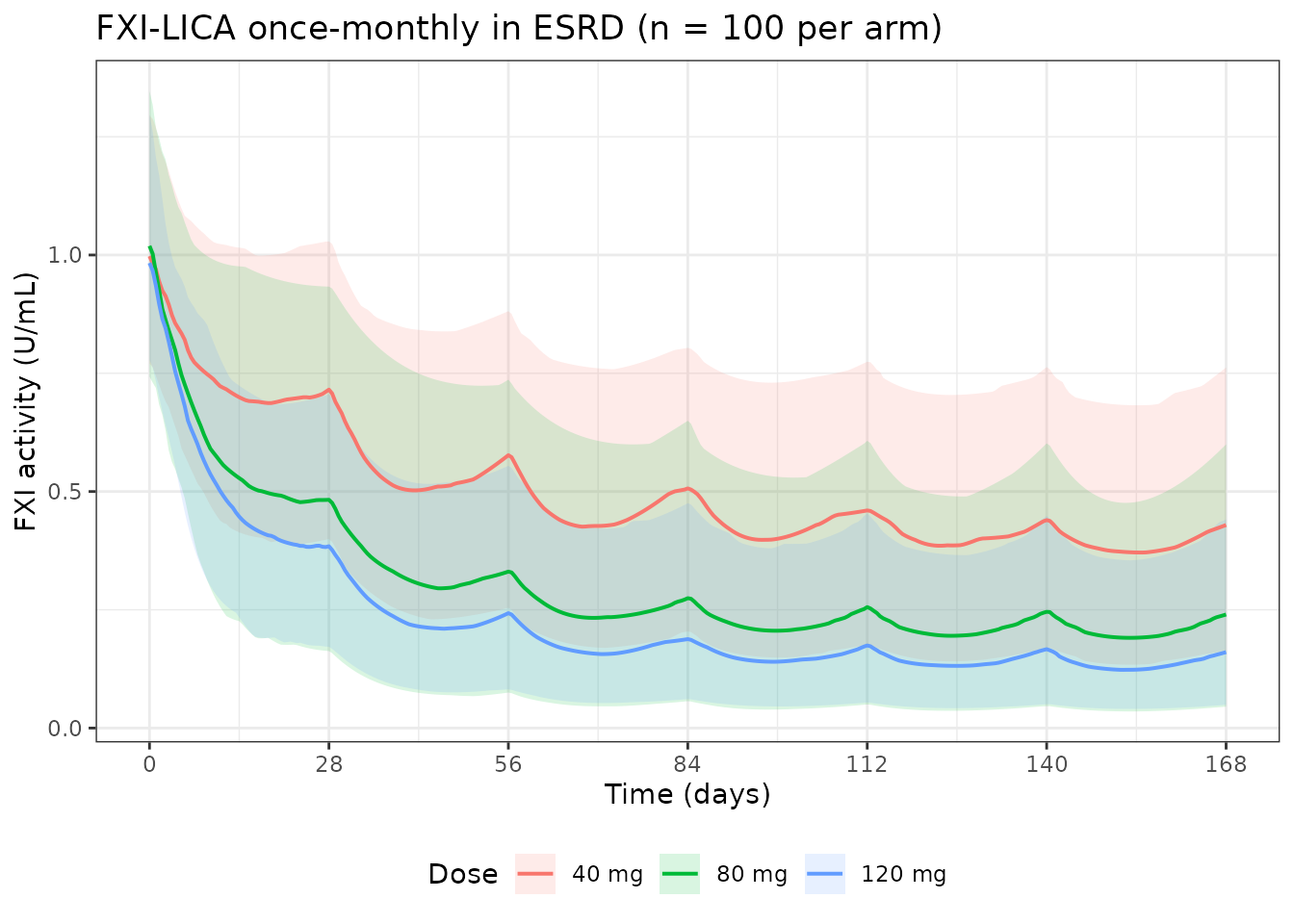

Replicates Figure 4a of Willmann 2021: model-predicted FXI activity time courses in ESRD patients after repeated once-monthly SC FXI-LICA at 40, 80, and 120 mg.

PKNCA validation: IONIS-FXIRX single 300 mg dose

Run PKNCA on the single-dose IONIS-FXIRX HV profile to sanity-check the simulated PK. Willmann 2021 does not report tabulated NCA values for IONIS-FXIRX, so this check verifies that AUC scales linearly with dose and $C_{max}$ is reasonable for a subcutaneous 2-cmt model with mixed absorption.

# Add extra observation rows to make PKNCA reliable, including t=0.
pknca_obs_times <- sort(unique(c(
  0, 0.25, 0.5, 0.75, 1, 1.5, 2, 3, 4, 6, 8, 10, 12, 16, 20, 24,
  36, 48, 72, 96, 120, 168, 240, 336, 504, 672, 840, 1008
)))

ionis_dose_levels <- c(50, 100, 200, 300)
subjects_ionis_nca <- data.frame(
  id = 100L + seq_along(ionis_dose_levels),
  wt = 70,
  esrd = 0,
  dose_mg = ionis_dose_levels
)
ev_ionis_nca <- make_events(
  subjects_ionis_nca,
  dose_times = 0,
  obs_times = pknca_obs_times
)

sim_ionis_nca <- rxode2::rxSolve(
  mod_ionis_typ, events = ev_ionis_nca,
  keep = c("WT", "RRT_HEMODIAL_STATUS", "dose_mg")
) |> as.data.frame()
#> ℹ omega/sigma items treated as zero: 'etalcl', 'etalvc', 'etalq', 'etalvp', 'etalka', 'etalogitfdepot', 'etalrbase', 'etalic50', 'etalkout', 'etalke0'
#> Warning: multi-subject simulation without without 'omega'

conc_obj <- PKNCA::PKNCAconc(
  data = dplyr::filter(sim_ionis_nca, !is.na(Cc)),
  formula = Cc ~ time | id / dose_mg
)
dose_df <- sim_ionis_nca |>
  dplyr::group_by(id) |>
  dplyr::summarize(
    time = 0,
    dose_mg = dplyr::first(dose_mg),
    .groups = "drop"
  ) |>
  dplyr::mutate(amt = dose_mg)
dose_obj <- PKNCA::PKNCAdose(
  data = dose_df,
  formula = amt ~ time | id
)
data_obj <- PKNCA::PKNCAdata(
  conc_obj, dose_obj,
  intervals = data.frame(
    start = 0, end = Inf,
    cmax = TRUE, tmax = TRUE, aucinf.obs = TRUE, half.life = TRUE
  )
)
res <- PKNCA::pk.nca(data_obj)

res_df <- as.data.frame(res$result)
res_summary <- res_df |>
  dplyr::filter(PPTESTCD %in% c("cmax", "tmax", "aucinf.obs", "half.life")) |>
  dplyr::select(dose_mg, PPTESTCD, PPORRES) |>
  tidyr::pivot_wider(names_from = PPTESTCD, values_from = PPORRES) |>
  dplyr::rename(
    `Dose (mg)`      = dose_mg,
    `Cmax (ng/mL)`   = cmax,
    `Tmax (h)`       = tmax,
    `AUCinf (ng*h/mL)` = aucinf.obs,
    `t1/2 (h)`       = half.life
  )
knitr::kable(res_summary, digits = 2,
             caption = "IONIS-FXIRX typical-value NCA parameters, single SC doses in a 70-kg HV.")

IONIS-FXIRX typical-value NCA parameters, single SC doses in a 70-kg HV.
Dose (mg)	Cmax (ng/mL)	Tmax (h)	t1/2 (h)	AUCinf (ng*h/mL)
50	1675.23	4	598.55	15836.69
100	3350.45	4	598.55	31673.38
200	6700.91	4	598.55	63346.77
300	10051.36	4	598.55	95020.14

Dose linearity check: for a linear system Cmax and AUCinf should scale approximately proportionally with dose.

PKNCA validation: FXI-LICA single doses

lica_dose_levels <- c(40, 60, 80, 120)
subjects_lica_nca <- data.frame(
  id = 500L + seq_along(lica_dose_levels),
  wt = 78,
  esrd = 0,
  dose_mg = lica_dose_levels
)
ev_lica_nca <- make_events(
  subjects_lica_nca,
  dose_times = 0,
  obs_times = pknca_obs_times
)

sim_lica_nca <- rxode2::rxSolve(
  mod_lica_typ, events = ev_lica_nca,
  keep = c("WT", "RRT_HEMODIAL_STATUS", "dose_mg")
) |> as.data.frame()
#> ℹ omega/sigma items treated as zero: 'etalcl', 'etalvc', 'etalq', 'etalvp', 'etalka', 'etalrbase', 'etalic50', 'etalkout', 'etalke0'
#> Warning: multi-subject simulation without without 'omega'

conc_obj_lica <- PKNCA::PKNCAconc(
  data = dplyr::filter(sim_lica_nca, !is.na(Cc)),
  formula = Cc ~ time | id / dose_mg
)
dose_df_lica <- sim_lica_nca |>
  dplyr::group_by(id) |>
  dplyr::summarize(time = 0, dose_mg = dplyr::first(dose_mg), .groups = "drop") |>
  dplyr::mutate(amt = dose_mg)
dose_obj_lica <- PKNCA::PKNCAdose(dose_df_lica, formula = amt ~ time | id)
data_obj_lica <- PKNCA::PKNCAdata(
  conc_obj_lica, dose_obj_lica,
  intervals = data.frame(
    start = 0, end = Inf,
    cmax = TRUE, tmax = TRUE, aucinf.obs = TRUE, half.life = TRUE
  )
)
res_lica <- PKNCA::pk.nca(data_obj_lica)
res_lica_df <- as.data.frame(res_lica$result) |>
  dplyr::filter(PPTESTCD %in% c("cmax", "tmax", "aucinf.obs", "half.life")) |>
  dplyr::select(dose_mg, PPTESTCD, PPORRES) |>
  tidyr::pivot_wider(names_from = PPTESTCD, values_from = PPORRES) |>
  dplyr::rename(
    `Dose (mg)`      = dose_mg,
    `Cmax (ng/mL)`   = cmax,
    `Tmax (h)`       = tmax,
    `AUCinf (ng*h/mL)` = aucinf.obs,
    `t1/2 (h)`       = half.life
  )
knitr::kable(res_lica_df, digits = 2,
             caption = "FXI-LICA typical-value NCA parameters, single SC doses in a 78-kg HV.")

FXI-LICA typical-value NCA parameters, single SC doses in a 78-kg HV.
Dose (mg)	Cmax (ng/mL)	Tmax (h)	t1/2 (h)	AUCinf (ng*h/mL)
40	338.63	2	402.12	3110.22
60	507.95	2	402.12	4665.34
80	677.26	2	402.12	6220.45
120	1015.89	2	402.12	9330.67

Assumptions and deviations

Reference weight for the BWT-on-V2 covariate is set to 70 kg in the IONIS-FXIRX model. Willmann 2021 Table S2 reports the exponent (BWT on V2 = 0.967) but does not state the reference weight; 70 kg is the standard NONMEM allometric-scaling reference and was chosen here to be consistent with the vast majority of popPK extractions in nlmixr2lib. An alternative (78 kg, the pooled ASO-CS1 + ASO-CS4 sample-size-weighted mean) would shift V2 for typical-weight subjects by only $$1.4% (0.978^0.967 vs 1.114^0.967), well below the parameter’s confidence interval (0.619-1.32).
Per-study residual error not simultaneously exposed. Willmann 2021 estimated study-specific proportional residual errors on both PK and PD (Tables S2 and S4). Each model file exposes ONE proportional SD per output (the healthy-volunteer study’s value in the IONIS-FXIRX file; the LICA-CS1 value in the FXI-LICA file). Users who need the ESRD-specific ASO-CS4 residual errors should override propSd = 0.290 and propSd_FXIact = 0.172 after loading Willmann_2021_ionisFxirx.
F1 IIV omitted from the FXI-LICA final model. Table S3 does not report an omega^2 on Logit(F1) for FXI-LICA (only 5 IIV rows on CL, V2, Q, V3, kA). This is faithful to the paper – the FXI-LICA model file uses a typical-value F1 for all subjects. The IONIS-FXIRX model file DOES include F1 IIV (omega^2 = 1.84 on the logit scale, %CV = 230) per Table S2.
ESRD covariates for FXI-LICA are BORROWED, not estimated. Willmann 2021 did not fit the ESRD covariates on FXI-LICA (only HV data available for FXI-LICA in the main analysis). For the paper’s FXI-LICA-in-ESRD simulations, the IONIS-FXIRX ESRD factors (CL x 0.470, V3 x 0.621, effect-site x 0.329) were transferred under the biological assumption that ESRD does not affect ASGPR-mediated hepatic uptake. This assumption is stated explicitly in the paper’s Methods and Discussion; the model file exposes the borrowed factors as fixed() parameters so the ESRD simulation scenario is reproducible.
Effect-compartment concentration scaling in units. The NONMEM control stream (Supplement 2, $DES) uses CONC = A(2)/V2 as the driving concentration and reports IC50 in ng/mL, which is consistent with a NONMEM dataset that converts doses to ug so that A(2)/V2 is in ug/L = ng/mL. In the nlmixr2 model here, the equivalent unit alignment is achieved by scaling central / vc (in mg/L) by 1000 before driving the effect compartment. The Errata bullet is a documentation artefact; the model is dimensionally correct.
RRT_HEMODIAL_STATUS covariate scoping. Willmann 2021 studied the effect of active hemodialysis sessions on IONIS-FXIRX PK/PD in a dedicated PK cohort (single 300 mg dose given immediately post- versus pre-dialysis) and concluded that hemodialysis itself did not alter the PK or PD. The covariate in this model is therefore the subject-level treatment-status indicator RRT_HEMODIAL_STATUS (per the canonical register), not the per-session indicator RRT_HEMODIAL_ACTIVE.
Original observed data are not publicly available; NCA comparisons in this vignette are simulated versus simulated (dose linearity), not simulated versus observed. The paper reports no side-by-side tabulated Cmax / Tmax / AUC values for the two ASOs, so a formal ncaComparisonTable() is not produced – the sanity checks confirm dose proportionality and expected orders of magnitude relative to reported doses.