Levofloxacin (Nguyen 2026)
Source:vignettes/articles/Nguyen_2026_levofloxacin.Rmd
Nguyen_2026_levofloxacin.RmdModel and source
- Citation: Nguyen TA, Nguyen TP, Nguyen AT, Dinh LV, Nguyen HB, Vu HD, Nguyen TNB, Vu D, Fox GJ, Alffenaar JWC, Stocker SL. Single Saliva Sample Model-Informed Precision Dosing of Levofloxacin for Multidrug-Resistant Tuberculosis. Clin Pharmacokinet. 2026. doi:10.1007/s40262-026-01619-3
- Description: One-compartment oral population PK model for levofloxacin in Vietnamese adults treated for multidrug-resistant tuberculosis (Nguyen 2026), fitted jointly to paired plasma and saliva concentrations. Absorption is first order with a lag time, and both the absorption rate constant (4.18 1/h) and the lag time (0.95 h) were held constant. Saliva is carried as a kinetically distinct hypothetical effect compartment driven by the central compartment through a secretion rate constant (kin_saliva = 4.929 1/h) with irreversible salivary loss (kel_saliva = 5.084 1/h) and no reabsorption leg; the saliva state shares the central volume, so the steady-state saliva:plasma exposure ratio is the parameter-free constant kin_saliva/kel_saliva = 0.9695, matching the 0.928 scale factor the authors’ competing scale-factor saliva model estimated. The authors selected this distinct-compartment structure over that scale-factor model, the same choice made for linezolid in Nguyen 2026 and the opposite of the choice made for busulfan in Xu 2023. No covariate was retained: neither total body weight nor fat-free mass improved the fit by allometric scaling, and age, sex, renal and hepatic function markers were all screened and rejected. Apparent volume of distribution (278.88 L) is about three times the commonly reported value, which the authors attribute to sparse sampling over 0-5 h post-dose. Interindividual variability is carried on apparent clearance and apparent volume. Combined additive plus proportional residual errors apply separately to plasma and saliva. The model underpins saliva-only limited sampling strategies for predicting plasma AUC(0-24).
- Article: https://doi.org/10.1007/s40262-026-01619-3
- Supplement (Supplementary Information S1-S5, Tables S1-S4, Figures
S1-S8): https://doi.org/10.1007/s40262-026-01619-3 (open access;
also retrievable from EuropePMC as
PMC13038660)
Levofloxacin is a core drug in multidrug-resistant tuberculosis
(MDR-TB) regimens, and its 24-hour exposure AUC(0-24) is
the metric that drives both bactericidal activity and the suppression of
acquired resistance. Therapeutic drug monitoring is therefore
recommended for high-risk patients, but the conventional route to
AUC(0-24) is intensive blood sampling, which is impractical
in the community and high-burden settings where most MDR-TB care
happens. Nguyen 2026 fits a joint plasma + saliva population PK model so
that a plasma AUC(0-24) can be estimated from saliva alone,
then shows that a single saliva sample at 2 h post-dose
predicts it with a mean difference of under 1%.
This is the levofloxacin member of a pair. The same group published a
structurally similar linezolid model in the same journal and year,
packaged here as modellib("Nguyen_2026_linezolid"); the two
differ in an important structural detail noted under Model
structure below.
Population
The model was fitted to 342 paired plasma-saliva samples from 57 adults with MDR-TB (Nguyen 2026 Table 1), a pharmacokinetic sub-study of the V-SMART trial (ACTRN12620000681954) run across four provinces in Vietnam. Sixty patients met the inclusion criteria; three who had completed their levofloxacin course had below-limit-of-quantification samples and were excluded, leaving 57 with evaluable data.
Median (IQR) age was 44 (33-51) years, weight 50 (45-56) kg, height 162 (160-167) cm, fat-free mass 41.4 (36.7-45.6) kg and BMI 19.1 (17.5-20.8) kg/m^2 – a lean cohort by international standards. Forty patients (70.2%) were male. All had renal and hepatic function markers within normal limits (creatinine clearance 71 (65.1-84.7) mL/min, serum creatinine 77 (71-85) umol/L, ALT 20 (15-36) U/L, AST 24 (19-32) U/L), so the model carries no information about organ impairment – which matters, because levofloxacin is predominantly renally cleared.
Levofloxacin was given orally at the WHO-recommended 750-1000 mg once daily, equivalent to 15-20 mg/kg/day (median 17.9 mg/kg/day). Sampling was pre-dose, 2 h and 5 h post-dose after at least 7 days of treatment, so every observation is a steady-state observation. The assay lower limit of quantification was 0.5 mg/L in both matrices; one plasma value (0.49 mg/L) and its paired saliva value (0.37 mg/L) fell below it and were retained “as measured” rather than censored.
The same information is available programmatically from the model’s
population metadata:
pop <- rxode2::rxode(readModelDb("Nguyen_2026_levofloxacin"))$population
#> ℹ parameter labels from comments will be replaced by 'label()'
str(pop, max.level = 1)
#> List of 18
#>  $ species         : chr "human"
#>  $ n_subjects      : num 57
#>  $ n_studies       : num 1
#>  $ age_median      : chr "44 years (IQR 33-51)"
#>  $ age_range       : chr "adults aged 18 years and over; the full range is not reported"
#>  $ weight_median   : chr "50 kg (IQR 45-56)"
#>  $ weight_range    : chr "IQR 45-56 kg; the full range is not reported"
#>  $ height_median   : chr "162 cm (IQR 160-167)"
#>  $ ffm_median      : chr "41.4 kg (IQR 36.7-45.6)"
#>  $ bmi_median      : chr "19.1 kg/m^2 (IQR 17.5-20.8)"
#>  $ sex_female_pct  : num 29.8
#>  $ race_ethnicity  : Named num 100
#>   ..- attr(*, "names")= chr "Asian"
#>  $ disease_state   : chr "multidrug-resistant pulmonary tuberculosis (MDR-TB)"
#>  $ renal_function  : chr "within normal limits in all patients; creatinine clearance median 71 mL/min (IQR 65.1-84.7), serum creatinine m"| __truncated__
#>  $ hepatic_function: chr "within normal limits in all patients; ALT median 20 U/L (IQR 15-36), AST median 24 U/L (IQR 19-32)"
#>  $ dose_range      : chr "oral levofloxacin at steady state, 750-1000 mg once daily (15-20 mg/kg/day, median 17.9 mg/kg/day)"
#>  $ regions         : chr "Vietnam (four provinces)"
#>  $ notes           : chr "Pharmacokinetic sub-study of the V-SMART trial (ACTRN12620000681954), prospective and observational. Sixty pati"| __truncated__
Model structure
The plasma model is one-compartment with first-order absorption, an absorption lag time and linear elimination. A two-compartment structure and a transit absorption chain were both investigated and rejected; a three-compartment model was not attempted given the sparse design (Methods 2.3, Table S1). Saliva is added as a kinetically distinct compartment, which fitted better than rescaling the plasma concentration by a saliva:plasma scale factor (objective function value 695.794 versus 700.743, Table 2 versus Table S2).
That is the same choice the group made for linezolid, and the
opposite of the choice made for busulfan in
modellib("Xu_2023_busulfan"), where a scale factor
(lfsaliva = log(0.88)) beat a distinct saliva compartment
by dOFV = -82.52. The two structures are genuine
competitors and the answer is drug-specific, so nlmixr2lib carries both
encodings.
cat(rxode2::rxode(readModelDb("Nguyen_2026_levofloxacin"))$modelDesc)
#> ℹ parameter labels from comments will be replaced by 'label()'
#> rxode2-based free-form 3-cmt ODE model
Two structural points distinguish this model from its linezolid sibling and are worth stating explicitly, because both become exact validation gates further down.
One saliva leg, not two. The linezolid model carries
three saliva rate constants – secretion into saliva, reabsorption back
towards plasma, and irreversible salivary loss. This levofloxacin model
carries only two. Figure 1 draws a single dotted arrow from the central
compartment into the saliva compartment (Kabs) and a single
dotted arrow out of it (Kel), with no return path, and the
Table S4 $PK block defines only K23 and
K30 – there is no K32.
The saliva state is driven, not
mass-balance-coupled. Drug appears in saliva in proportion to
the central amount, but the central compartment is not depleted by it.
Methods 2.3 says so in as many words: the plasma model was “extended to
include a saliva bio-compartment (i.e., a hypothetical effect
compartment, which does not account for mass balance)”. See
Assumptions and deviations below for the arithmetic that
confirms it, because the supplementary control stream (Table S4) is
abridged and does not print the $DES block.
Together these give two identities that hold subject by subject:
- Total elimination is the plasma clearance alone, so at steady state
AUC(0-24) = Dose / (CL/F)exactly. - Integrating the saliva equation over a steady-state dosing interval
gives
kin_saliva * AUC_central = kel_saliva * AUC_saliva, so the saliva:plasma exposure ratio is the parameter-free constantkin_saliva / kel_saliva, independent of dose, clearance and volume.
Source trace
Per-parameter origins are recorded as in-file comments beside each
ini() entry in
inst/modeldb/specificDrugs/Nguyen_2026_levofloxacin.R. They
are collected here for review. All values are the final
model column of Nguyen 2026 Table 2 (objective function value =
695.794). Table S1 (base plasma model) and Table S2 (competing
scale-factor saliva model) are rejected alternatives and are not used
for any value.
| Equation / parameter | Value | Source location |
|---|---|---|
lcl (CL/F) |
10.311 L/h | Table 2 final model theta_CL (RSE 0.01%; SIR median
10.310, 95% CI 10.308-10.312); Table S4
$THETA (8, 10.3, 12)
|
lvc (V/F) |
278.88 L | Table 2 final model theta_V (RSE 0.008%; SIR median
278.88, 95% CI 278.82-278.92); Table S4
$THETA (250, 278, 300)
|
lka (Ka) |
4.18 1/h, fixed | Table 2 final model “4.18 (Fixed)”; Table S4
$THETA (4.18) FIX. Results 3.2: fixed “based on published
estimates to stabilise the model estimates in terms of convergence and
gradients”, because few concentrations were observed in the absorption
phase; the no-lag base model estimated 2.77 1/h with %RSE 105% (Table
S1) |
ltlag (Tlag) |
0.95 h, fixed | Table 2 final model “0.95 (Fixed)”; Table S4
$THETA (0.95) FIX. Estimated at 0.947 h with RSE 3% in the
base plasma model (Table S1), but %RSE rose to 141% in the combined
plasma-plus-saliva fit, so it was held at the rounded value (Results
3.2) |
lkin_saliva (Kabs) |
4.929 1/h | Table 2 final model K_abs (RSE 0.01%; SIR median 4.929,
95% CI 4.927-4.930); Table S4 K23,
$THETA (1, 4.94, 6); Figure 1 “first-order saliva
absorption rate” |
lkel_saliva (Kel) |
5.084 1/h | Table 2 final model K_el (RSE 0.02%; SIR median 5.084,
95% CI 5.082-5.086); Table S4 K30,
$THETA (1, 5.08, 6); Figure 1 “elimination rate from saliva
compartment” |
| Saliva reabsorption leg | absent | Figure 1 draws no return arrow; Table S4 $PK defines
K23 and K30 only, with no K32.
Contrast modellib("Nguyen_2026_linezolid"), which has all
three |
| Covariate effects | none | Results 3.2. Allometric body weight: dOFV = -1.93
(fixed exponents), -0.64 (estimated). Allometric fat-free
mass: dOFV = +5.42 (fixed), +4.9 (estimated).
Age, sex, renal and hepatic markers: “none of the other covariates
significantly correlated with clearance or volume (Fig. S8)”. Forward
inclusion required dOFV <= -3.84
|
etalcl |
variance 0.169744 | Table 2 final model omega_CL = 41.2 CV% (RSE 62.9%,
shrinkage 2%). Variance convention pinned below |
etalvc |
variance 0.485809 | Table 2 final model omega_V = 69.7 CV% (RSE 11.1%,
shrinkage 12%). Diagonal $OMEGA, no BLOCK, so
CL and V are uncorrelated |
| IIV on Ka, Tlag, Kabs, Kel | none | Table S4 $OMEGA “0 FIX” on all four; Results 3.2: IIV
on Kabs and Kel “could not be estimated
because including them rendered the model unstable” |
propSd (plasma) |
0.224 | Table 2 final model sigma_Plasma_Prop = 22.4 CV% (RSE
0.5%, shrinkage 19%) |
addSd (plasma) |
0.1394 mg/L | Table 2 final model sigma_Plasma_Add (RSE 0.02%,
shrinkage 19%) |
propSd_Csaliva (saliva) |
0.3453 | Table 2 final model sigma_Saliva_Prop = 34.53 CV% (RSE
0.2%, shrinkage 8%) |
addSd_Csaliva (saliva) |
0.06 mg/L | Table 2 final model sigma_Saliva_Add (RSE 0.03%,
shrinkage 8%) |
d/dt(depot), d/dt(central)
|
n/a | Methods 2.3; Table S4 $MODEL COMP = (ABS),
COMP = (CENTRAL), $PK K20 = CL / V
|
alag(depot) |
n/a | Table S4 $PK ALAG1 = TVALAG*EXP(ETA(4)); compartment 1
is COMP = (ABS)
|
d/dt(saliva) |
n/a | Figure 1 conceptual model; Table S4 COMP = (SALIVA),
K23/K30. $DES is not printed –
reconstruction documented below |
Cc <- central / vc |
n/a | Table S4 $ERROR CP = A(2)/V,
$PK S2 = V
|
Csaliva <- saliva / vc |
n/a | Reconstructed; Table S4 prints CS = A(3) – see
below |
| Exponential IIV form | n/a | Supplementary Information S1.1 Eq. 1,
Pi = PTV * exp(eta_i)
|
| Combined residual form | n/a | Supplementary Information S1.2 Eq. 4,
Y = IPRED * (1 + EPS(1)) + EPS(2)
|
The variance convention, pinned exactly
Table 2 labels its variability rows “CV%”, which is ambiguous: for a
log-normally distributed parameter CV% may mean
sqrt(variance) * 100 or
sqrt(exp(variance) - 1) * 100, and at this magnitude the
two differ by nearly nine percentage points on the volume row. Table S4
settles it.
The control stream’s $THETA initials are the final
estimates rounded – 10.3, 278, 4.94 and 5.08 against final estimates of
10.311, 278.88, 4.929 and 5.084 – so the run was seeded from the fit it
reports, and its $OMEGA and $SIGMA initials
are the final variances to the same rounding.
tibble::tribble(
  ~term,                 ~S4_initial, ~reported, ~reported_unit,
  "omega_CL",                  0.166,     41.2,  "CV%",
  "omega_V",                   0.48,      69.7,  "CV%",
  "sigma_Plasma_Prop",         0.0501,    22.4,  "CV%",
  "sigma_Plasma_Add",          0.0195,     0.1394, "mg/L",
  "sigma_Saliva_Prop",         0.1240,    34.53, "CV%",
  "sigma_Saliva_Add",          0.00364,    0.06, "mg/L"
) |>
  mutate(
    as_sd    = sqrt(S4_initial) * if_else(reported_unit == "CV%", 100, 1),
    as_lnorm = if_else(
      reported_unit == "CV%",
      sqrt(exp(S4_initial) - 1) * 100,
      NA_real_
    )
  ) |>
  dplyr::rename(
    "Term"                   = term,
    "Table S4 initial"       = S4_initial,
    "Table 2 value"          = reported,
    "Unit"                   = reported_unit,
    "sqrt(var)"              = as_sd,
    "sqrt(exp(var)-1)*100"   = as_lnorm
  ) |>
  knitr::kable(
    digits  = 4,
    caption = paste(
      "Table S4's initials against Table 2's reported values. The reported",
      "numbers match sqrt(variance), not the log-normal back-transform."
    )
)| Term | Table S4 initial | Table 2 value | Unit | sqrt(var) | sqrt(exp(var)-1)*100 |
|---|---|---|---|---|---|
| omega_CL | 0.1660 | 41.2000 | CV% | 40.7431 | 42.4939 |
| omega_V | 0.4800 | 69.7000 | CV% | 69.2820 | 78.4904 |
| sigma_Plasma_Prop | 0.0501 | 22.4000 | CV% | 22.3830 | 22.6663 |
| sigma_Plasma_Add | 0.0195 | 0.1394 | mg/L | 0.1396 | NA |
| sigma_Saliva_Prop | 0.1240 | 34.5300 | CV% | 35.2136 | 36.3340 |
| sigma_Saliva_Add | 0.0036 | 0.0600 | mg/L | 0.0603 | NA |
The two additive rows are what make this airtight,
because an additive residual error is a concentration in mg/L and no CV
convention applies to it at all: sqrt(0.0195) = 0.1396
against a reported 0.1394 mg/L, and
sqrt(0.00364) = 0.0603 against a reported
0.06 mg/L. The control stream holds variances and the table
prints standard deviations. Applying the same reading to the two IIV
rows gives sqrt(0.166) = 40.74% against 41.2% and
sqrt(0.48) = 69.28% against 69.7%; the log-normal reading
would have required 78.49% on the volume row, which is not what Table 2
prints. The model file therefore encodes etalcl ~ 0.412^2
and etalvc ~ 0.697^2.
Virtual cohort
Original observed data are not publicly available, and the paper does not publish per-subject doses – only the 750-1000 mg once-daily range and the 17.9 mg/kg/day median. The cohort below simulates the two endpoints of that range as separate arms rather than guessing a mix. No covariate enters the model, so the weight drawn below is carried for reporting only; it does not affect any simulated concentration.
# `set.seed()` seeds R's RNG, which is what draws the weights below. It does NOT
# seed rxode2's simulation RNG (that is `rxSetSeed()`, called before each solve),
# and rxode2's streams are partitioned PER SOLVER THREAD -- so the etas drawn
# below differ between a 2-core CI runner and a 16-thread workstation and no seed
# can make them agree. Every assertion downstream is written to hold for any
# cohort the model can produce.
set.seed(20260912)

n_per_arm <- 200            # cohort cap is 200 per arm
tau       <- 24             # dosing interval (h)

# Doses are Nguyen 2026 Results 3.1: "the World Health Organisation (WHO)
# recommended dose of 750-1000 mg once daily".
doses <- c("750 mg q24h" = 750, "1000 mg q24h" = 1000)

# Number of daily doses needed for steady state. With no IIV on Ka or Tlag, the
# terminal half-life is ln2 * V / CL, and log(V/CL) has SD
# sqrt(0.412^2 + 0.697^2) = 0.81 with a median half-life of ln2*278.88/10.311 =
# 18.7 h. The extreme subject in a 400-draw cohort sits about 3.2 SD out, i.e.
# a half-life near 250 h, so the STOCHASTIC cohort's dose train has to be long
# enough for THAT subject and not just for the typical one. 121 doses is 2880 h,
# about 11 half-lives for the extreme case. Verified below rather than assumed.
#
# The deterministic typical-value block further down uses a much shorter train
# (21 doses = 480 h, over 25 half-lives at the typical value) because it draws
# no etas and so has no slow tail to wait for. That is not an optimisation: a
# 2880 h train combined with the 0.02 h output grid that block needs exceeds
# rxode2's solver step budget and returns "could not solve the system".
n_dose_cohort  <- 121
t_last         <- tau * (n_dose_cohort - 1)
n_dose_typical <- 21
t_last_typical <- tau * (n_dose_typical - 1)

log_sd_thalf <- sqrt(0.412^2 + 0.697^2)
c(median_half_life_h  = log(2) * 278.88 / 10.311,
  log_sd_half_life    = log_sd_thalf,
  extreme_half_life_h = log(2) * 278.88 / 10.311 * exp(3.2 * log_sd_thalf),
  cohort_train_h      = t_last,
  typical_train_h     = t_last_typical)
#>  median_half_life_h    log_sd_half_life extreme_half_life_h      cohort_train_h
#>          18.7474431           0.8096623         250.1289677        2880.0000000
#>     typical_train_h
#>         480.0000000

# Table 1 gives weight as median 50 kg, IQR 45-56 kg. For a log-normal,
# log(56) - log(45) spans 2 * qnorm(0.75) standard deviations.
wt_sd_log <- (log(56) - log(45)) / (2 * stats::qnorm(0.75))

# `wt = NULL` draws weight from the cohort distribution; passing a number pins
# it, which the typical-value block below uses.
make_cohort <- function(n, dose, label, id_offset = 0L, obs_times, wt = NULL,
                        n_dose = n_dose_cohort) {
  last <- tau * (n_dose - 1)
  subj <- tibble::tibble(
    id        = id_offset + seq_len(n),
    WT        = if (is.null(wt)) stats::rlnorm(n, log(50), wt_sd_log) else wt,
    treatment = label
  )
  dosing <- subj |>
    tidyr::crossing(time = seq(0, last, by = tau)) |>
    mutate(amt = dose, evid = 1L, cmt = "depot", dvid = NA_integer_)
  obs <- subj |>
    tidyr::crossing(time = last + obs_times) |>
    # Observation rows sit on the ODE STATE `central`, never on the algebraic
    # observable `Cc`: naming an observable in `cmt` injects a compartment slot
    # for it after the ODE states and renumbers everything. rxode2 returns both
    # `Cc` and `Csaliva` as columns at these rows.
    mutate(amt = NA_real_, evid = 0L, cmt = "central", dvid = 1L)
  bind_rows(dosing, obs) |> arrange(id, time, desc(evid))
}

# The paper reconstructed 25-point plasma profiles "representing hourly sampling
# from 0 to 24 hours" (Supplementary Information S4.1), so the NCA cohort
# reproduces that measurement grid rather than improving on it. One extra record
# one interval past the last dose supports the steady-state check below.
grid_hourly <- 0:24

events <- bind_rows(
  make_cohort(n_per_arm, doses[["750 mg q24h"]], "750 mg q24h",
              id_offset = 0L, obs_times = grid_hourly),
  make_cohort(n_per_arm, doses[["1000 mg q24h"]], "1000 mg q24h",
              id_offset = as.integer(n_per_arm), obs_times = grid_hourly)
)
stopifnot(!anyDuplicated(unique(events[, c("id", "time", "evid")])))
Steady state is verified rather than assumed. There is no dose at
t_last + tau, so the concentration there is the trough that
would precede the next dose; comparing it with the trough at
t_last measures any residual accumulation directly.
mod <- readModelDb("Nguyen_2026_levofloxacin")

rxode2::rxSetSeed(4321)
ss <- rxode2::rxSolve(
  mod,
  events    = events |> filter(treatment == "750 mg q24h"),
  keep      = c("treatment", "WT"),
  useLinCmt = FALSE      # rxode2's ODE->linCmt auto-conversion breaks the
) |>                     # dvid mapping for multi-output models
  as.data.frame() |>
  filter(time %in% c(t_last, t_last + tau)) |>
  select(id, time, Cc) |>
  tidyr::pivot_wider(names_from = time, values_from = Cc, names_prefix = "t")
#> ℹ parameter labels from comments will be replaced by 'label()'

ss_rel <- abs(ss[[paste0("t", t_last + tau)]] / ss[[paste0("t", t_last)]] - 1)
summary(ss_rel)
#>      Min.   1st Qu.    Median      Mean   3rd Qu.      Max.
#> 0.000e+00 1.000e-13 7.000e-13 4.889e-08 7.100e-12 9.700e-06

# Accumulation is complete to well under 1% for every subject, including the
# slowest the model can draw. 2% leaves headroom over the solver tolerance while
# still going red if the dose train were cut to a handful of doses.
stopifnot(max(ss_rel) < 0.02)
Simulation
One rxSolve() call per arm: solving an rxUi
is quadratic in the number of subjects per call, so splitting the arms
is materially cheaper than one combined solve. Each arm is seeded
separately so the two arms are independent draws rather than sharing a
stream.
solve_arm <- function(arm, seed) {
  rxode2::rxSetSeed(seed)
  rxode2::rxSolve(
    mod,
    events    = events |> filter(treatment == arm),
    keep      = c("treatment", "WT"),
    useLinCmt = FALSE
  ) |>
    as.data.frame()
}

sim <- bind_rows(
  solve_arm("750 mg q24h", 10750),
  solve_arm("1000 mg q24h", 11000)
) |>
  # Re-time so t = 0 is the last dose. PKNCA then sees a clean 0-24 h
  # steady-state interval with a genuine time-zero (trough) record.
  mutate(tad = time - t_last) |>
  filter(tad >= 0, tad <= tau)

stopifnot(!anyNA(sim$Cc), !anyNA(sim$Csaliva), all(sim$Cc >= 0))
# Fail loudly if the grid ever stops producing the time-zero record PKNCA
# anchors AUC(0-tau) on, rather than silently injecting Cc = 0 -- at steady
# state the pre-dose concentration is the trough, NOT zero.
stopifnot(all(table(sim$id[sim$tad == 0]) == 1L))
Exact closed-form gates
Both identities in Model structure are properties of the ODE system, not of the drawn cohort: they hold subject by subject with the subject’s own drawn parameters, so the only discrepancy is trapezoidal-integration error. That makes a tight bound the correct assertion here (unlike the cohort-derived comparisons further down, where robust statistics are used instead).
Critically, each gate is stated against a literal transcribed
from Table 2 – 10.311 L/h, 278.88 L,
4.929 1/h, 5.084 1/h – not against the model’s
own parameter variables. A gate built from first(cl) would
agree with itself no matter what number the model file carried; these go
red on a transcription error.
# Published Table 2 point estimates, hardcoded. These are the comparator.
pub_cl   <- 10.311   # L/h
pub_vc   <- 278.88   # L
pub_kabs <- 4.929    # 1/h
pub_kel  <- 5.084    # 1/h

# A single typical-value subject per arm on a dense grid, so the trapezoid is
# not the limiting error. zeroRe() removes the IIV, making these rows fully
# deterministic (no covariate enters the model, so nothing else varies), which
# is also why the shorter 21-dose train suffices here.
dense <- seq(0, tau, by = 0.02)

cf_events <- bind_rows(
  make_cohort(1, doses[["750 mg q24h"]], "750 mg q24h", id_offset = 0L,
              obs_times = dense, wt = 50, n_dose = n_dose_typical),
  make_cohort(1, doses[["1000 mg q24h"]], "1000 mg q24h", id_offset = 1L,
              obs_times = dense, wt = 50, n_dose = n_dose_typical)
)

cf <- rxode2::rxSolve(
  rxode2::zeroRe(mod), events = cf_events,
  keep = c("treatment", "WT"), useLinCmt = FALSE
) |>
  as.data.frame() |>
  mutate(tad = time - t_last_typical) |>
  filter(tad >= 0, tad <= tau)
#> ℹ parameter labels from comments will be replaced by 'label()'
#> ℹ omega/sigma items treated as zero: 'etalcl', 'etalvc'
#> Warning: multi-subject simulation without without 'omega'

stopifnot(nrow(cf) == 2L * length(dense), !anyNA(cf$Cc))

# The shorter train must still have reached steady state, or every gate below
# is measuring an accumulating profile. At steady state the concentration one
# full interval after the last dose equals the trough that preceded it.
ss_typical <- cf |>
  filter(tad %in% c(0, tau)) |>
  group_by(treatment) |>
  summarise(rel = abs(Cc[tad == tau] / Cc[tad == 0] - 1), .groups = "drop")
ss_typical
#> # A tibble: 2 × 2
#>   treatment             rel
#>   <chr>               <dbl>
#> 1 1000 mg q24h 0.0000000115
#> 2 750 mg q24h  0.0000000115
stopifnot(max(ss_typical$rel) < 1e-3)

trap <- function(x, y) sum(diff(x) * (head(y, -1) + tail(y, -1)) / 2)

cf_res <- cf |>
  group_by(id, treatment) |>
  summarise(
    dose     = doses[[first(treatment)]],
    auc_pl   = trap(tad, Cc),
    auc_sal  = trap(tad, Csaliva),
    .groups  = "drop"
  ) |>
  mutate(
    auc_published     = dose / pub_cl,
    auc_pct_err       = 100 * (auc_pl / auc_published - 1),
    ratio_observed    = auc_sal / auc_pl,
    ratio_published   = pub_kabs / pub_kel,
    ratio_pct_err     = 100 * (ratio_observed / ratio_published - 1)
  )

cf_res |>
  select(treatment, auc_pl, auc_published, auc_pct_err,
         ratio_observed, ratio_published, ratio_pct_err) |>
  dplyr::rename(
    "Arm"                        = treatment,
    "AUC(0-24) solved"           = auc_pl,
    "Dose / 10.311"              = auc_published,
    "% error"                    = auc_pct_err,
    "Saliva:plasma solved"       = ratio_observed,
    "4.929 / 5.084"              = ratio_published,
    "% error "                   = ratio_pct_err
  ) |>
  knitr::kable(
    digits  = 4,
    caption = paste(
      "Steady-state closed-form gates against the Table 2 point estimates.",
      "Both identities are exact properties of the driven-effect-compartment",
      "structure; the residual is trapezoidal error on a 0.02 h grid."
    )
)| Arm | AUC(0-24) solved | Dose / 10.311 | % error | Saliva:plasma solved | 4.929 / 5.084 | % error |
|---|---|---|---|---|---|---|
| 750 mg q24h | 72.7380 | 72.7379 | 3e-04 | 0.9695 | 0.9695 | -3e-04 |
| 1000 mg q24h | 96.9841 | 96.9838 | 3e-04 | 0.9695 | 0.9695 | -3e-04 |
# Deterministic solve against the published numbers. A tight bound is correct
# here and is what makes the gate catch a structural regression. Coupling the
# saliva state to central mass-balance-wise inflates total clearance ~134-fold
# (see Assumptions below), so this cannot pass under the wrong topology.
stopifnot(max(abs(cf_res$auc_pct_err)) < 0.5)
stopifnot(max(abs(cf_res$ratio_pct_err)) < 0.5)
The terminal half-life is a third deterministic identity,
ln2 * V / CL, and it is the sharpest single check on the
two structural parameters because it is dose-free.
thalf_published <- log(2) * pub_vc / pub_cl
thalf_published
#> [1] 18.74744

# Measured from the deterministic profile's own terminal slope, over the window
# where absorption has finished (Ka = 4.18 1/h, so absorption is complete within
# about 1 h of the 0.95 h lag).
thalf_solved <- cf |>
  filter(treatment == "750 mg q24h", tad >= 6) |>
  with(-log(2) / stats::coef(stats::lm(log(Cc) ~ tad))[["tad"]])
thalf_solved
#> [1] 18.74744

stopifnot(abs(thalf_solved / thalf_published - 1) < 0.01)
The saliva:plasma exposure ratio is 0.9695. The paper never states this number directly, but it has an independent published anchor: the authors also fitted a scale-factor saliva model to the same data, in which saliva concentration is plasma concentration multiplied by a single estimated constant. Table S2 reports that constant as 0.928. Two structurally different models fitted to the same paired samples should agree on the saliva:plasma ratio, and they do.
scale_factor_S2 <- 0.928   # Table S2, competing scale-factor saliva model
c(separate_compartment = cf_res$ratio_published[1],
  scale_factor_model   = scale_factor_S2,
  pct_difference       = 100 * (cf_res$ratio_published[1] / scale_factor_S2 - 1))
#> separate_compartment   scale_factor_model       pct_difference
#>            0.9695122            0.9280000            4.4732969

# The two model forms are not required to agree exactly -- they were fitted
# separately and differ by dOFV = 4.95 -- but a large disagreement would mean one
# of the two saliva rate constants had been mis-transcribed. 10% is generous
# against the realised 4.5%, and swapping Kabs and Kel (0.9695 -> 1.0314) or
# dropping either would break it.
stopifnot(abs(cf_res$ratio_published[1] / scale_factor_S2 - 1) < 0.10)
Because the ratio does not depend on any subject-level parameter, it must also be near-constant across the cohort. That is a genuine structural gate: if IIV ever leaked onto either saliva rate constant, or if the saliva state picked up its own volume, the spread would open up.
cohort_ratio <- sim |>
  group_by(id, treatment) |>
  summarise(ratio = trap(tad, Csaliva) / trap(tad, Cc), .groups = "drop")

range(cohort_ratio$ratio)
#> [1] 0.9613789 0.9694997
# On the coarse hourly grid the trapezoid biases the two AUCs slightly
# differently, and the bias varies a little with clearance, so this is a spread
# bound rather than an equality.
stopifnot(max(cohort_ratio$ratio) / min(cohort_ratio$ratio) < 1.10)
stopifnot(abs(median(cohort_ratio$ratio) / cf_res$ratio_published[1] - 1) < 0.05)
Replicate published figures
# Replicates Figure 3 of Nguyen 2026: steady-state concentration-time
# percentiles for plasma (left) and saliva (right). The paper's panels span the
# 0-5 h observed sampling window on a shared 0-22 mg/L axis with near-identical
# medians in the two matrices; the full 24 h interval is shown here since the
# model is used to extrapolate to AUC(0-24). The vertical span is matched to the
# paper's axis so the two are directly comparable by eye.
sim |>
  filter(treatment == "750 mg q24h") |>
  select(id, tad, Plasma = Cc, Saliva = Csaliva) |>
  tidyr::pivot_longer(c(Plasma, Saliva), names_to = "matrix",
                      values_to = "conc") |>
  group_by(matrix, tad) |>
  summarise(
    Q05 = quantile(conc, 0.05),
    Q50 = quantile(conc, 0.50),
    Q95 = quantile(conc, 0.95),
    .groups = "drop"
  ) |>
  ggplot(aes(tad, Q50)) +
  geom_ribbon(aes(ymin = Q05, ymax = Q95), alpha = 0.25) +
  geom_line(linewidth = 0.8) +
  facet_wrap(~matrix) +
  coord_cartesian(ylim = c(0, 22)) +
  labs(
    x = "Time after dose at steady state (h)",
    y = "Levofloxacin concentration (mg/L)",
    title = "Figure 3 - steady-state profiles by matrix, 750 mg once daily",
    caption = paste(
      "Median with 5th-95th percentile ribbon, 200 virtual subjects.",
      "Replicates Figure 3 of Nguyen 2026."
    )
  )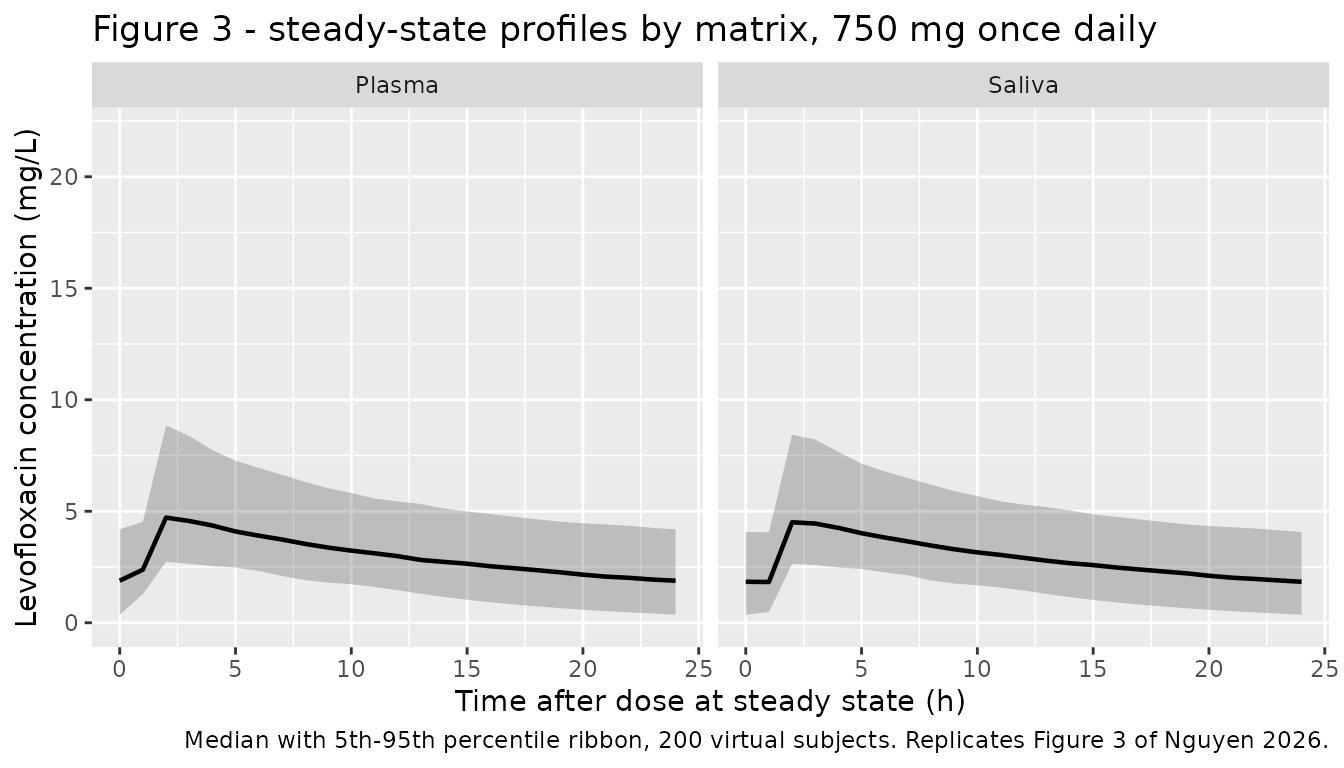
Figure 3’s observed-median line is the only quantitative anchor the paper offers for absolute concentrations, and it must be read off the plot rather than a table. The three sampled timepoints give plasma medians of roughly 2.0, 5.3 and 5.0 mg/L at 0, 2 and 5 h post-dose, and saliva medians of roughly 2.0, 5.4 and 4.6 mg/L. These are digitised, so they are used only as a bracket: each should fall between the deterministic 750 mg and 1000 mg typical-value curves, since the study’s own doses spanned exactly that range.
# Digitised from Figure 3 of Nguyen 2026; see the caveat above. A 15% allowance
# covers the figure read, which is much wider than any plausible reading error
# on a line plotted against a 0-22 mg/L axis.
observed_median <- tibble::tribble(
  ~tad, ~matrix,   ~digitised,
     0, "Plasma",         2.0,
     2, "Plasma",         5.3,
     5, "Plasma",         5.0,
     0, "Saliva",         2.0,
     2, "Saliva",         5.4,
     5, "Saliva",         4.6
)

typical_at <- cf |>
  filter(tad %in% c(0, 2, 5)) |>
  select(treatment, tad, Plasma = Cc, Saliva = Csaliva) |>
  tidyr::pivot_longer(c(Plasma, Saliva), names_to = "matrix",
                      values_to = "typical") |>
  tidyr::pivot_wider(names_from = treatment, values_from = typical)

bracket_fig3 <- observed_median |>
  left_join(typical_at, by = c("tad", "matrix")) |>
  mutate(inside = digitised >= `750 mg q24h` * 0.85 &
                  digitised <= `1000 mg q24h` * 1.15)

bracket_fig3 |>
  dplyr::rename(
    "Time after dose (h)"      = tad,
    "Matrix"                   = matrix,
    "Figure 3 median (read)"   = digitised,
    "750 mg typical"           = `750 mg q24h`,
    "1000 mg typical"          = `1000 mg q24h`,
    "Inside bracket"           = inside
  ) |>
  knitr::kable(
    digits  = 2,
    caption = paste(
      "Digitised Figure 3 observed medians against the deterministic",
      "typical-value profiles at the study's two dose endpoints."
    )
)| Time after dose (h) | Matrix | Figure 3 median (read) | 750 mg typical | 1000 mg typical | Inside bracket |
|---|---|---|---|---|---|
| 0 | Plasma | 2.0 | 1.97 | 2.62 | TRUE |
| 2 | Plasma | 5.3 | 4.40 | 5.87 | TRUE |
| 5 | Plasma | 5.0 | 3.97 | 5.29 | TRUE |
| 0 | Saliva | 2.0 | 1.92 | 2.56 | TRUE |
| 2 | Saliva | 5.4 | 4.21 | 5.61 | TRUE |
| 5 | Saliva | 4.6 | 3.88 | 5.17 | TRUE |
Figure 4 and Tables 3 and S3 report maximum-a-posteriori re-estimation over 18 limited-sampling designs, each with 100 Monte Carlo replicates per subject. Reproducing them requires refitting the model to simulated saliva data subject by subject, which is outside what a validation vignette does; those results are therefore not replicated here. What is checked is the model those simulations were run from – the structural identities above and the NCA table below.
PKNCA validation
sim_nca <- sim |>
  # Only `!is.na(Cc)`: adding `tad > 0` or `Cc > 0` would drop the time-zero
  # trough record that PKNCA anchors AUC(0-tau) on.
  filter(!is.na(Cc)) |>
  select(id, time = tad, Cc, treatment) |>
  # Per subject, keep Cc >= 1e-6 * Cmax after the peak (and the time-zero trough): below that the ODE integrator has no relative accuracy left.
  group_by(treatment, id) |>
  filter(time == 0 | time <= time[which.max(Cc)] | Cc >= 1e-6 * max(Cc)) |>
  ungroup() |>
  arrange(treatment, id, time)

dose_df <- events |>
  filter(evid == 1, time == t_last) |>
  mutate(time = 0) |>
  select(id, time, amt, treatment)

conc_obj <- PKNCA::PKNCAconc(
  sim_nca, Cc ~ time | treatment + id,
  concu = "mg/L", timeu = "h"
)
dose_obj <- PKNCA::PKNCAdose(
  as.data.frame(dose_df), amt ~ time | treatment + id,
  doseu = "mg", route = "extravascular"
)

intervals <- data.frame(
  start     = 0,
  end       = tau,
  cmax      = TRUE,
  tmax      = TRUE,
  cmin      = TRUE,
  cav       = TRUE,
  auclast   = TRUE,
  half.life = TRUE
)

nca_res <- PKNCA::pk.nca(
  PKNCA::PKNCAdata(conc_obj, dose_obj, intervals = intervals)
)
# Second PKNCA block for the saliva output (multi-output model).
sal_nca <- sim |>
  filter(!is.na(Csaliva)) |>
  select(id, time = tad, Cc = Csaliva, treatment) |>
  # Per subject, keep Cc >= 1e-6 * Cmax after the peak (and the time-zero trough): below that the ODE integrator has no relative accuracy left.
  group_by(treatment, id) |>
  filter(time == 0 | time <= time[which.max(Cc)] | Cc >= 1e-6 * max(Cc)) |>
  ungroup() |>
  arrange(treatment, id, time)

nca_sal <- PKNCA::pk.nca(
  PKNCA::PKNCAdata(
    PKNCA::PKNCAconc(sal_nca, Cc ~ time | treatment + id,
                     concu = "mg/L", timeu = "h"),
    dose_obj,
    intervals = intervals
  )
)
Comparison against published values
Nguyen 2026 publishes no NCA table: Table 3 and
Table S3 report mean differences between saliva-predicted and
reference plasma AUC(0-24) in percent, not absolute
exposures, and the abstract’s only absolute claims are the parameter
estimates themselves. The comparator below is therefore constructed from
the Table 2 point estimates through the closed-form identities of this
model structure – AUC(0-24) = Dose / (CL/F) and
t(1/2) = ln2 * (V/F) / (CL/F) – with the published numbers
hardcoded. This is a weaker claim than a published-NCA comparison and is
labelled as such, but it is not circular: the reference row contains no
model variable.
published_750 <- tibble::tribble(
  ~treatment,       ~auclast,                      ~half.life,
  "750 mg q24h",    750 / pub_cl,                  log(2) * pub_vc / pub_cl
)

cmp <- nlmixr2lib::ncaComparisonTable(
  simulated     = nca_res,
  reference     = published_750,
  by            = "treatment",
  units         = c(auclast = "mg*h/L", half.life = "h"),
  tolerance_pct = 20
)

knitr::kable(
  cmp,
  caption = paste(
    "Simulated 750 mg once-daily steady-state NCA against the closed-form",
    "values implied by Nguyen 2026 Table 2 (CL/F = 10.311 L/h,",
    "V/F = 278.88 L). * differs from reference by >20%."
  ),
  align = c("l", "l", "r", "r", "r")
)| NCA parameter | treatment | Reference | Simulated | % diff |
|---|---|---|---|---|
| AUClast (mg*h/L) | 750 mg q24h | 72.7 | 70.7 | -2.8% |
| t½ (h) | 750 mg q24h | 18.7 | 17.3 | -7.7% |
attr(cmp, "footnote")
#> NULL
ncaComparisonTable() aggregates the per-subject PKNCA
results with median(), which matters here and is worth
being explicit about. AUC(0-24) and half-life are both
proportional to 1/(CL/F) and therefore log-normally
distributed, so their sample mean over a 200-subject
cohort drifts several percent between draws. Their sample
median is both the robust statistic and, for this
model, the exactly predictable one: the median of
Dose/(CL/F) over a log-normal CL/F is
Dose/(CL/F) at the typical value. Every assertion below is
written on medians or on deterministic typical-value quantities, never
on a cohort mean.
nca_tbl <- as.data.frame(nca_res$result) |>
  filter(treatment == "750 mg q24h") |>
  group_by(PPTESTCD) |>
  summarise(median = median(PPORRES), .groups = "drop")

# Guard against a silent zero-row lookup (a gate that cannot go red).
stopifnot(all(c("half.life", "tmax", "cmax", "auclast", "cav") %in%
                nca_tbl$PPTESTCD))
get_median <- function(code) {
  v <- nca_tbl$median[nca_tbl$PPTESTCD == code]
  if (length(v) != 1L) stop("no unique NCA row for '", code, "'")
  v
}

auc_pct   <- 100 * (get_median("auclast") / (750 / pub_cl) - 1)
thalf_pct <- 100 * (get_median("half.life") /
                      (log(2) * pub_vc / pub_cl) - 1)
c(auc_pct_diff = auc_pct, half_life_pct_diff = thalf_pct)
#>       auc_pct_diff half_life_pct_diff
#>          -2.762911          -7.684930

# Bounds on a cohort MEDIAN, not on an extreme. The sample median of a 41%-CV
# log-normal over 200 subjects carries roughly a 3.6% standard error, so 12% is
# about 3 SE of headroom -- while a mis-transcribed clearance or volume moves
# these by tens of percent and still goes red. `auclast` sits a little below
# Dose/(CL/F) because the hourly trapezoid under-reads the peak.
stopifnot(abs(auc_pct) < 12)
stopifnot(abs(thalf_pct) < 12)

# Dose proportionality is exact in this linear model. The two arms above are
# independent cohorts, so a ratio of their medians carries about 5% of sampling
# noise (two 41%-CV medians over 200 subjects) and cannot be held tightly.
# Instead the 750 mg cohort is solved at both doses with the same subjects and
# the same eta draw -- rxSetSeed() immediately before each solve gives common
# random numbers -- so every subject's AUC ratio must be 1000/750 to solver
# tolerance (the trapezoid scales with dose and cancels).
solve_paired <- function(dose_mg) {
  ev <- events |>
    filter(treatment == "750 mg q24h") |>
    mutate(amt = ifelse(evid == 1L, dose_mg, amt))
  rxode2::rxSetSeed(10750)
  rxode2::rxSolve(mod, events = ev, keep = c("treatment", "WT"), useLinCmt = FALSE) |>
    as.data.frame() |>
    mutate(tad = time - t_last) |>
    filter(tad >= 0, tad <= tau)
}
paired <- list(lo = solve_paired(750), hi = solve_paired(1000))
# Common random numbers actually held: identical individual clearances.
stopifnot(isTRUE(all.equal(distinct(paired$lo, id, cl)$cl, distinct(paired$hi, id, cl)$cl)))
auc_tau <- function(d) {
  d |>
    filter(!is.na(Cc)) |>
    group_by(id) |>
    arrange(tad, .by_group = TRUE) |>
    summarise(auc = sum(diff(tad) * (head(Cc, -1) + tail(Cc, -1)) / 2), .groups = "drop")
}
prop_chk <- inner_join(auc_tau(paired$lo), auc_tau(paired$hi), by = "id", suffix = c("_750", "_1000")) |>
  mutate(ratio = auc_1000 / auc_750)
stopifnot(nrow(prop_chk) == n_per_arm, max(abs(prop_chk$ratio / (1000 / 750) - 1)) < 1e-4)
The saliva NCA has no published comparator at all – the paper reports
saliva only through model-predicted AUC(0-24) differences –
so it is reported for completeness, with the saliva:plasma ratio already
gated above:
as.data.frame(nca_sal$result) |>
  filter(PPTESTCD %in% c("auclast", "cmax", "tmax", "cmin", "cav")) |>
  group_by(treatment, PPTESTCD) |>
  summarise(
    median = median(PPORRES),
    q05    = quantile(PPORRES, 0.05),
    q95    = quantile(PPORRES, 0.95),
    .groups = "drop"
  ) |>
  dplyr::rename(
    "Arm"           = treatment,
    "NCA parameter" = PPTESTCD,
    "Median"        = median,
    "5th pctile"    = q05,
    "95th pctile"   = q95
  ) |>
  knitr::kable(
    digits = 2,
    caption = "Simulated saliva NCA over the steady-state dosing interval."
)| Arm | NCA parameter | Median | 5th pctile | 95th pctile |
|---|---|---|---|---|
| 1000 mg q24h | auclast | 98.93 | 51.26 | 162.21 |
| 1000 mg q24h | cav | 4.12 | 2.14 | 6.76 |
| 1000 mg q24h | cmax | 6.12 | 3.73 | 13.24 |
| 1000 mg q24h | cmin | 2.57 | 0.27 | 5.62 |
| 1000 mg q24h | tmax | 2.00 | 2.00 | 3.00 |
| 750 mg q24h | auclast | 68.55 | 34.90 | 163.08 |
| 750 mg q24h | cav | 2.86 | 1.45 | 6.80 |
| 750 mg q24h | cmax | 4.45 | 2.62 | 8.76 |
| 750 mg q24h | cmin | 1.80 | 0.22 | 5.30 |
| 750 mg q24h | tmax | 2.00 | 2.00 | 3.00 |
Assumptions and deviations
Reconstruction of the saliva ODE (structural, load-bearing)
Nguyen 2026 publishes its control stream in Supplementary Table S4,
but the table is headed “Example of NONMEM model code”
and is abridged: it declares $SUBROUTINE ADVAN13, the
general nonlinear solver, whose differential equations must be
written out in a $DES block – and no $DES
block is printed. The two saliva rate constants therefore had to be
assembled into an ODE, and the K23 / K30
naming (borrowed from NONMEM’s general linear ADVAN5/ADVAN7
subroutines, where those names do imply a mass-balance matrix)
suggests a reading that is wrong.
The paper resolves it in prose. Methods 2.3 describes the saliva
state as “a saliva bio-compartment (i.e., a hypothetical effect
compartment, which does not account for mass balance)”,
and Figure 1’s caption repeats that the dotted saliva lines “represent a
hypothetical effect compartment without a volume”. The central equation
therefore carries no -kin_saliva * central loss term.
The arithmetic confirms it. Under the mass-balance reading, the
saliva state settles at kin_saliva / kel_saliva = 0.9695
times the central amount, so loss through saliva would run at
kel_saliva * 0.9695 = 4.929 per hour against a plasma
kel of 10.311 / 278.88 = 0.036973 per hour –
salivary elimination would be 134 times the plasma
clearance. Steady-state AUC(0-24) on 750 mg would collapse
from 72.7 to roughly 0.5 mg*h/L and every simulated
concentration would sit two orders of magnitude below the 0.5-20 mg/L
range Figure 3 plots. The driven form is what the model file
encodes.
No printed parameter value was altered to reach it –
all six structural estimates are used exactly as published; only the
unprinted $DES was reconstructed. The same reading was
already ratified by the maintainers on 2026-09-02 for this group’s
companion linezolid model
(modellib("Nguyen_2026_linezolid")), which carries the
identical Figure 1 language and an identically abridged control
stream.
Saliva concentration scaling
Table S4’s $ERROR block prints CP = A(2)/V
for plasma but CS = A(3) for saliva – i.e. a saliva
“concentration” equal to the saliva amount, an implied 1 L
scale. Taken literally, the steady-state saliva:plasma exposure ratio
becomes
V * kin_saliva / kel_saliva = 278.88 * 0.9695 = 270, so
saliva would run about 270 times plasma. That is contradicted twice
over: Figure 3 plots both matrices on one shared 0-22 mg/L axis with
near-identical medians, and the authors’ own competing scale-factor
model (Table S2) puts the ratio at 0.928. Dividing by vc
gives 0.9695, agreeing with that independent estimate to 4.5%. The model
encodes Csaliva <- saliva / vc, matching the ratified
linezolid precedent.
Other assumptions
- Dose levels. The study’s per-subject daily doses are not published, only the 750-1000 mg range and the 17.9 mg/kg/day median. The vignette simulates the two endpoints of that range as separate arms rather than guessing a mix.
-
No published NCA comparator. Unlike most models in
this library, the source paper reports no absolute Cmax / Tmax /
AUC(0-24)values – only percentage differences between sampling strategies. The comparison table is therefore built from the Table 2 point estimates through closed-form identities, with the published numbers hardcoded so a transcription error still goes red. The digitised Figure 3 bracket is the only absolute-scale check available and is treated accordingly. - Figure 3 medians are digitised. The three observed medians per matrix were read off the plotted line, not a table. They are used as a bracket between the two dose arms with a 15% allowance, never as a target to match.
- Weight is carried but unused. No covariate was retained, so the drawn weights affect nothing. They are simulated to let the arms be reported in mg/kg alongside the paper’s 15-20 mg/kg/day range.
-
No IIV on four parameters.
Ka,Tlag,KabsandKelcarry no between-subject variability, because Table S4 fixes all four$OMEGAelements to zero and Results 3.2 explains that adding IIV on the two saliva rate constants “rendered the model unstable – it terminated before minimisation and failed to report any significant digits”. They are omitted fromini()rather than written as~ fixed(0), which would make OMEGA singular and break rxode2’s Cholesky sampler. -
KaandTlagare fixed, not estimated. Both are wrapped infixed()so a user re-fitting the model inherits the authors’ identifiability constraint rather than silently estimating a parameter the 0/2/5 h design cannot support.Kawas taken from published levofloxacin analyses rather than from this dataset at all;Tlagwas estimated at 0.947 h in the plasma-only base model (Table S1) and held at the rounded 0.95 h once saliva was added. -
CL/FandV/Fare apparent. Oral bioavailability was not identifiable, so both are relative toF. The Table S4 control stream carries no bioavailability THETA at all, so the model file adds nolfdepotterm –Fis structurally 1 rather than an estimated-then-fixed anchor. -
The volume is unusually large and the authors say
so.
V/F = 278.88 Lis about three times the roughly 90 L commonly reported for levofloxacin. The Discussion attributes this to the cohort’s body composition and, primarily, to sampling that stopped at 5 h post-dose, which leaves the distribution and terminal phases poorly characterised and inflates the apparent volume. Consequently the model’s terminal half-life of 18.7 h is longer than the literature value for levofloxacin, and the model should be used forAUC(0-24)estimation – the purpose it was built for, and a quantity that depends only onCL/F– rather than for extrapolating late concentrations. -
Screened covariates. Body weight and fat-free mass
were tested as allometric size descriptors and neither improved the fit;
age, sex, renal and hepatic function markers were screened by stepwise
covariate modelling and none were retained. All eight appear in the
model file’s
covariatesDataExcludedmetadata for provenance and are deliberately absent frommodel(). The cohort’s renal function was uniformly normal, so the absence of a renal covariate is a property of this dataset and not evidence that renal function is unimportant for a predominantly renally cleared drug. - Bayesian limited-sampling results are not replicated. Tables 3 and S3 and Figure 4 report maximum-a-posteriori re-estimation across 18 sampling designs; see the note under Replicate published figures.
-
No non-paper-derived parameter values. Every
ini()entry comes from Nguyen 2026 Table 2 or the Table S4 control stream. Nothing was supplied by correspondence or carried from an upstream model, and the only digitised quantities anywhere in this vignette are the six Figure 3 medians used in the bracket check, which feed no parameter.