Meropenem (Butragueno-Laiseca 2024)

Model and source

ui <- rxode2::rxode(readModelDb("ButraguenoLaiseca_2024_meropenem"))
#> ℹ parameter labels from comments will be replaced by 'label()'

Citation: Butragueno-Laiseca L, Troconiz IF, Grau S, Campillo N, Padilla B, Fernandez SN, Slocker M, Herrera L, Santiago MJ. How to use meropenem in pediatric patients undergoing CKRT? Integrated meropenem pharmacokinetic model for critically ill children. Antimicrob Agents Chemother. 2024;68(6):e0172923. doi:10.1128/aac.01729-23
Description: Two-compartment population PK model for intravenous meropenem in 16 critically ill children in a paediatric ICU, 7 of whom were receiving continuous kidney replacement therapy (CKRT) (Butragueno-Laiseca 2024). Five matrices were fitted simultaneously following the Broeker et al. approach – plasma, pre-filter, post-filter, effluent and urine – which untangles total elimination into three additive arms: a renal arm (CLR, 5.5 L/h at full maturity and a median eGFR of 95 mL/min/1.73 m2, encoded as lcl_renal), a non-renal / metabolic arm (CLM, 0.91 L/h, encoded as lcl_nonren) and a CKRT arm (CLCKRT, 1.26 L/h for the medium hemofilter, encoded as lcl_hemodialysis). The renal arm scales linearly with eGFR and carries a postnatal-age maturation function reaching half of the mature value at 15.6 months (Hill coefficient not significantly different from 1); in CKRT patients it is replaced by a flat 0.96 L/h for those retaining residual diuresis and switched off entirely in anuric patients. Hemofilter surface area is a categorical covariate on the CKRT arm (medium 0.6 m2 is the reference; low 0.2 m2 multiplier 0.27, high 1.2 m2 multiplier 1.5). Central volume scales linearly with body weight; the peripheral volume and the inter-compartmental clearance carry no covariates and no IIV. Post-filter and effluent concentrations are derived algebraically from the pre-filter (central) concentration using the measured circuit blood and effluent flows, and the urinary concentration from a cumulative urinary-amount state divided by the collected volume; each of the four observables carries its own log-scale residual error.
Article: https://doi.org/10.1128/aac.01729-23
Open-access record: PMC11620509

This is the meropenem companion of the already-packaged ButraguenoLaiseca_2025_teicoplanin model: the same group, the same paediatric intensive care unit, the same Prismaflex CKRT circuit and the same pre-filter / post-filter algebra. The meropenem analysis goes two matrices further, adding the effluent and urine compartments, and it is that addition which lets the authors split total elimination into three arms that a plasma-only design cannot separate.

Population

Sixteen critically ill children treated with meropenem in a single paediatric intensive care unit (Hospital General Universitario Gregorio Maranon, Madrid) were enrolled; seven of them were undergoing continuous kidney replacement therapy (CKRT). Median (IQR) age was 8 (3.5-82) months without CKRT and 48 (5-106) months with CKRT, and median (IQR) weight 7.5 (5.5-17.5) kg and 20 (7.4-40) kg respectively; neither difference was statistically significant (Butragueno-Laiseca 2024 Table 1). Most patients (62.5%) were in the postoperative period of congenital cardiopathy. Illness severity was higher in the CKRT group (PRISM III median 15 versus 5.5, P = 0.026). Neonates under 28 days of postnatal age were excluded.

All patients received 40 mg/kg of meropenem intravenously every 8 h as a 30-min infusion; in CKRT patients the interval was extended to every 12 h from the fourth dose, following the conventional renal adjustment. Sampling began after at least three doses, with blood and urine collected before (T0) and 2, 4, 6 and 8 h after the start of the infusion; CKRT patients additionally had pre-filter, post-filter and effluent samples drawn simultaneously, giving 18 samples each. A total of 212 concentrations were modelled - 99 plasma / pre-filter, 38 post-filter, 26 effluent and 49 urine, 60% of them from CKRT patients - none below the 0.5 mg/L limit of quantification.

Four of the seven CKRT patients were anuric; the other three passed 10-123 mL of urine over the PK sampling window. That split is what identifies the separate CKRT renal clearance discussed below.

The same information is available programmatically via the model’s population metadata:

str(ui$population, max.level = 1)
#> List of 15
#>  $ species       : chr "human"
#>  $ n_subjects    : int 16
#>  $ n_studies     : int 1
#>  $ n_observations: int 212
#>  $ age_range     : chr "3 to 173 months (supplemental Table S1); neonates under 28 days of postnatal age were excluded"
#>  $ age_median    : chr "8 months (IQR 3.5-82) without CKRT; 48 months (IQR 5-106) with CKRT"
#>  $ weight_range  : chr "not reported directly; IQR 5.5-17.5 kg without CKRT and 7.4-40 kg with CKRT"
#>  $ weight_median : chr "7.5 kg without CKRT; 20 kg with CKRT; 10 kg pooled (Table 4 footnote)"
#>  $ sex_female_pct: chr "Not reported."
#>  $ race_ethnicity: chr "Not reported."
#>  $ disease_state : chr "Critically ill children admitted to a paediatric intensive care unit and treated with meropenem, 7 of them unde"| __truncated__
#>  $ dose_range    : chr "Hospital protocol: 40 mg/kg intravenously every 8 h. In patients with CKRT the dosing interval was increased to"| __truncated__
#>  $ regions       : chr "Hospital General Universitario Gregorio Maranon, Madrid, Spain (single centre)."
#>  $ renal_function: chr "Group without CKRT: eGFR median 89 (IQR 69-122) mL/min/1.73 m^2, urine output median 1,100 (719-1,150) mL, hour"| __truncated__
#>  $ notes         : chr "Baseline demographics from Butragueno-Laiseca 2024 Table 1, reported separately for the 9 patients without and "| __truncated__

Source trace

The per-parameter origin is recorded as an in-file comment next to each ini() entry in inst/modeldb/specificDrugs/ButraguenoLaiseca_2024_meropenem.R. The table below collects them in one place for review.

Equation / parameter	Value	Source location
`lcl_renal` (theta_CLR)	5.5 L/h	Table 4 (RSE 13%); Results, Selection of covariates (“CLR for a patient with normal and fully mature renal function is 5.5 L/h”)
`tm50_cl_renal` (theta_50)	15.6 months	Table 4 (RSE 16%; SIR 95% CI 11.3-20)
`e_rrt_crrt_active_cl_renal` (theta_CLR_CKRT)	0.96 L/h	Table 4 (RSE 53%; SIR 95% CI 0.5-1.8)
`lcl_nonren` (theta_CLM)	0.91 L/h	Table 4 (RSE 25%; SIR 95% CI 0.6-1.3)
`lcl_hemodialysis` (theta_CLCKRT)	1.26 L/h	Table 4 (RSE 19%; SIR 95% CI 0.9-1.6), medium 0.6 m2 filter
`e_filt_sa_small_cl_hemodialysis` (theta_FILT_Low)	0.27	Table 4 (RSE 22%)
`e_filt_sa_large_cl_hemodialysis` (theta_FILT_High)	1.5	Table 4 (RSE 23%)
theta_FILT_Med = 1 (reference)	1	Table 4 and its footnote (filter surfaces 0.2 / 0.6 / 1.2 m2)
`lvc` (theta_V1)	4.75 L	Table 4 (RSE 17%; SIR 95% CI 3.6-5.9)
`e_wt_vc`	1 (fixed)	Table 4 Parameter model column, `theta_V1 x WGT/10`
reference weight	10 kg	Table 4 footnote (“WGT, body weight (median = 10 kg)”)
reference eGFR	95 mL/min/1.73 m2	Table 4 footnote (“eGFR … (median = 95 mL/min/1.73 m2)”)
`lvp` (theta_VT)	10.7 L	Table 4 (RSE 41%; SIR 95% CI 6.6-17.6)
`lq` (theta_CLD)	0.28 L/h	Table 4 (RSE 25%; SIR 95% CI 0.22-0.39)
`etalcl_renal`	30% CV	Table 4 IPV column (RSE 60%; SIR 95% CI 12-51; eta-shrinkage 43%)
`etalcl_nonren`	86% CV	Table 4 IPV column (RSE 59%; SIR 95% CI 60-122; eta-shrinkage 18%)
`etalvc`	48% CV	Table 4 IPV column (RSE 30%; SIR 95% CI 33-62; eta-shrinkage 14%)
omega^2 = log(1 + CV^2)	n/a	Table 4 footnote (CV% = sqrt(exp(omega^2) - 1) x 100)
No IIV on CLCKRT / CLD / V2; no eta covariance	n/a	Table 4 (“NS”); Results, Base population model
`expSd`	0.38	Table 4, plasma and prefilter residual error (RSE 12%)
`expSd_Cpostfilter`	0.38	Table 4, postfilter residual error (RSE 30%)
`expSd_Ceffluent`	0.37	Table 4, effluent residual error (RSE 36%)
`expSd_Curine`	0.86	Table 4, urine residual error (RSE 13%)
Log-additive residual -> `lnorm()`	n/a	Methods, PK analysis (“residual error was characterized with an additive model on the logarithmic scale”)
Two-compartment structure	n/a	Methods equations 1-2; Results, Base population model (1-cmt worse P < 0.001; 3-cmt no improvement)
`d/dt(urine) <- cl_renal * Cc`	n/a	Methods, equation 3
`Curine <- urine / UVol`	n/a	Methods, Base population model (“CUr was obtained as AUr/UVol”)
`Cpostfilter = Cc * (1 - CLCKRT / phi_Pl,corr)`	n/a	Methods, equation 4
`Ceffluent = CLCKRT * Cc / phi_Effl`	n/a	Methods, equation 5
`phi_Pl,corr = phi_Blood x (1 - Hct)`	n/a	Methods, equation 4 text plus Results, Base population model (BPR “equal to 1 [-] hematocrit”)
30-min IV infusion	n/a	Results, Probability of target attainment (“short infusion of 30 min”)

Structural checks

Every check below is a deterministic consequence of the encoded ini() values, recomputed and compared against a statement the paper makes about its own model. No simulation is involved, so these are exact transcription tests: a mis-transcribed theta breaks them immediately.

th <- ui$theta

theta_clr      <- exp(th[["lcl_renal"]])
theta_50       <- exp(th[["tm50_cl_renal"]])
theta_clr_ckrt <- th[["e_rrt_crrt_active_cl_renal"]]
theta_clm      <- exp(th[["lcl_nonren"]])
theta_clckrt   <- exp(th[["lcl_hemodialysis"]])
theta_v1       <- exp(th[["lvc"]])
theta_v2       <- exp(th[["lvp"]])
filt_low       <- th[["e_filt_sa_small_cl_hemodialysis"]]
filt_high      <- th[["e_filt_sa_large_cl_hemodialysis"]]

ref_wt   <- 10   # Table 4 footnote
ref_egfr <- 95   # Table 4 footnote

# Renal clearance for a patient NOT on CKRT (Table 4 parameter model).
clr_no_ckrt <- function(pna_months, egfr = ref_egfr) {
  theta_clr * (egfr / ref_egfr) * pna_months / (pna_months + theta_50)
}

Disposition volumes

v1_10kg <- theta_v1 * (10 / ref_wt)^th[["e_wt_vc"]]
vss     <- v1_10kg + theta_v2

# Discussion: "the resulting total apparent volume of distribution was 15.4 L"
# for the 10 kg typical patient, and Table 4's V1 is 4.75 L.
stopifnot(
  isTRUE(all.equal(v1_10kg, 4.75)),
  abs(vss - 15.4) < 0.05
)
c(V1_10kg = v1_10kg, Vss = vss)
#> V1_10kg     Vss 
#>    4.75   15.45

Clearance decomposition, patients without CKRT

The paper compares its typical patient against Saito et al.: “the total apparent volume of central compartment distribution and total clearances obtained by Saito et al. were 4.9 L and 4.6 L/h, in agreement with the estimates listed in Table 4 (4.75 L and 3.93 L/h)”. The 3.93 L/h reproduces exactly - but at a postnatal age of 19 months, not the 42 months the same sentence states. Both are shown so the discrepancy is visible rather than hidden; see Errata.

total_cl_no_ckrt <- function(pna_months, egfr = ref_egfr) {
  clr_no_ckrt(pna_months, egfr) + theta_clm
}

tibble::tibble(
  `Postnatal age (months)` = c(19, 42),
  `CLR (L/h)`    = clr_no_ckrt(c(19, 42)),
  `CLM (L/h)`    = theta_clm,
  `Total CL (L/h)` = total_cl_no_ckrt(c(19, 42)),
  Note = c(
    "cohort median age implied by supplemental Table S1; reproduces the published 3.93 L/h",
    "the age the Discussion sentence states"
  )
) |>
  dplyr::mutate(dplyr::across(where(is.numeric), \(x) signif(x, 3))) |>
  knitr::kable(caption = "Total clearance of the typical non-CKRT patient at the eGFR median of 95 mL/min/1.73 m2.")

Total clearance of the typical non-CKRT patient at the eGFR median of 95 mL/min/1.73 m2.
Postnatal age (months)	CLR (L/h)	CLM (L/h)	Total CL (L/h)	Note
19	3.02	0.91	3.93	cohort median age implied by supplemental Table S1; reproduces the published 3.93 L/h
42	4.01	0.91	4.92	the age the Discussion sentence states


# The published 3.93 L/h is quoted to three significant figures.
stopifnot(abs(total_cl_no_ckrt(19) - 3.93) < 0.005)

The eGFR effect is a bare normalisation

Two independent statements in the paper pin the eGFR term to a linear, through-origin normalisation by the cohort median of 95 mL/min/1.73 m2, which is why the model carries no estimated coefficient on it.

# Results: "an increment in eGFR of 10 mL/min/1.73 m2 is associated with a
# 10.5% increase in CLR."
pct_up_10 <- 100 * (clr_no_ckrt(19, ref_egfr + 10) / clr_no_ckrt(19, ref_egfr) - 1)

# Discussion: "The predicted percentage decreases in renal and total clearances
# for every reduction in 20 mL/min/1.73 m2 predicted by our model are 21% and
# 18%." The renal figure holds at any age; the total figure holds in the
# fully-mature limit, where CLR is at its 5.5 L/h asymptote.
pct_dn_renal <- 100 * (1 - clr_no_ckrt(19, ref_egfr - 20) / clr_no_ckrt(19, ref_egfr))
pct_dn_total <- 100 * (1 - (theta_clr * (ref_egfr - 20) / ref_egfr + theta_clm) /
                             (theta_clr + theta_clm))

tibble::tibble(
  Statement = c(
    "+10 mL/min/1.73 m2 raises CLR by (%)",
    "-20 mL/min/1.73 m2 lowers CLR by (%)",
    "-20 mL/min/1.73 m2 lowers total CL by (%), fully mature"
  ),
  Model     = c(pct_up_10, pct_dn_renal, pct_dn_total),
  Published = c(10.5, 21, 18),
  Source    = c("Results, Selection of covariates", "Discussion", "Discussion")
) |>
  dplyr::mutate(Model = round(Model, 2)) |>
  knitr::kable(caption = "Published eGFR sensitivities recomputed from the encoded model.")

Published eGFR sensitivities recomputed from the encoded model.
Statement	Model	Published	Source
+10 mL/min/1.73 m2 raises CLR by (%)	10.53	10.5	Results, Selection of covariates
-20 mL/min/1.73 m2 lowers CLR by (%)	21.05	21.0	Discussion
-20 mL/min/1.73 m2 lowers total CL by (%), fully mature	18.06	18.0	Discussion


stopifnot(
  abs(pct_up_10    - 10.5) < 0.05,
  abs(pct_dn_renal - 21)   < 0.5,
  abs(pct_dn_total - 18)   < 0.5
)

Maturation

# Results: "50% of adult renal function is achieved at the age of 15.9 months"
# (Table 4 prints theta_50 = 15.6 - see Errata) and Discussion: "90% of adult
# kidney functionality is predicted at ages over 12 months".
age_at_50 <- theta_50                       # by construction of the Emax form
age_at_90 <- 9 * theta_50                   # AGE/(AGE + T50) = 0.9

tibble::tibble(
  `Fraction of mature CLR` = c(0.5, 0.9),
  `Postnatal age (months)` = c(age_at_50, age_at_90),
  Published = c("15.6 (Table 4) / 15.9 (text)", "'over 12 months' (Discussion)")
) |>
  knitr::kable(caption = "Renal maturation milestones implied by the encoded theta_50.")

Renal maturation milestones implied by the encoded theta_50.
Fraction of mature CLR	Postnatal age (months)	Published
0.5	15.6	15.6 (Table 4) / 15.9 (text)
0.9	140.4	‘over 12 months’ (Discussion)


stopifnot(abs(age_at_50 - 15.6) < 0.05)

The Discussion’s “90% of adult kidney functionality is predicted at ages over 12 months” is not reproduced by the encoded maturation function, which needs 140 months to reach 90%; 12 months corresponds to 43% of the mature value. The sentence is better read as a loose statement about the clinical age above which renal maturation stops driving the dose, not as an evaluation of the printed equation.

Clearance decomposition, patients on CKRT

This is the paper’s central claim, and it is where the model structure is most strongly constrained by the text. The CKRT renal arm is flat at 0.96 L/h and is gated by residual diuresis; the extracorporeal arm scales with filter size.

clckrt <- c(
  "Low (0.2 m2)"    = theta_clckrt * filt_low,
  "Medium (0.6 m2)" = theta_clckrt,
  "High (1.2 m2)"   = theta_clckrt * filt_high
)

ckrt_share <- tibble::tibble(
  Filter        = names(clckrt),
  `CLCKRT (L/h)` = as.numeric(clckrt),
  `CLR (L/h)`    = theta_clr_ckrt,
  `CLM (L/h)`    = theta_clm,
  `Total CL (L/h)` = theta_clr_ckrt + theta_clm + as.numeric(clckrt),
  `CLCKRT share (%)` = 100 * as.numeric(clckrt) /
    (theta_clr_ckrt + theta_clm + as.numeric(clckrt)),
  Published = c(15, 40, 78)
)

ckrt_share |>
  dplyr::mutate(dplyr::across(where(is.numeric), \(x) round(x, 1))) |>
  knitr::kable(caption = "Extracorporeal share of total clearance in a CKRT patient with residual diuresis, versus the percentages stated in the Discussion.")

Extracorporeal share of total clearance in a CKRT patient with residual diuresis, versus the percentages stated in the Discussion.
Filter	CLCKRT (L/h)	CLR (L/h)	CLM (L/h)	Total CL (L/h)	CLCKRT share (%)	Published
Low (0.2 m2)	0.3	1	0.9	2.2	15.4	15
Medium (0.6 m2)	1.3	1	0.9	3.1	40.3	40
High (1.2 m2)	1.9	1	0.9	3.8	50.3	78


# The low- and medium-filter percentages reproduce to the printed digit. The
# high-filter figure does not: the model's own numbers give 50%, not 78%. It is
# reported here rather than accommodated -- see Errata.
stopifnot(
  abs(ckrt_share$`CLCKRT share (%)`[1] - 15) < 0.5,
  abs(ckrt_share$`CLCKRT share (%)`[2] - 40) < 0.5
)

# Results: "The depurative efficiency of the extracorporeal elimination was
# reduced and augmented by 73% and 50%, respectively, for low and high surface
# area filters compared to middle size."
stopifnot(
  abs(100 * (1 - filt_low)  - 73) < 0.5,
  abs(100 * (filt_high - 1) - 50) < 0.5
)

# Discussion: "for those patients that show diuresis, the estimate of renal
# clearance was five to sixfold lower than the corresponding value obtained in
# case of no CKRT".
fold <- theta_clr / theta_clr_ckrt
stopifnot(fold > 5, fold < 6)
round(fold, 2)
#> [1] 5.73

The anuria gate is confirmed by the paper’s own arithmetic

The paper never states in so many words that the 0.96 L/h renal arm applies only to CKRT patients who retain diuresis, and that anuric patients have no renal elimination at all. Two sentences imply it - “For the three patients under CKRT with diuresis, CLR was 0.96 L/h” and “for those patients that show diuresis, the estimate of renal clearance was five to sixfold lower” - and the Discussion’s comparison against Thy et al. confirms it arithmetically, because the two percentages it quotes are only recovered if the anuric arm has CLR = 0:

For the case of total clearance, an estimate of 1.34 L/h is associated with a patient with 10 kg of body weight, 4 years of age, and 1,200 mL/h of Qeff based on the model selected by Thy et al. That value is 37% and 56% lower than the corresponding values obtained from the current investigation in patients with CKRT and with or without diuresis.

thy_cl <- 1.34

# Medium (0.6 m2) filter, which is the size a 10 kg patient sits at the boundary
# of; it is the only choice that recovers both published percentages.
cl_with_diuresis    <- theta_clr_ckrt + theta_clm + theta_clckrt
cl_without_diuresis <- 0              + theta_clm + theta_clckrt

pct_lower <- 100 * (1 - thy_cl / c(cl_with_diuresis, cl_without_diuresis))

tibble::tibble(
  `CKRT patient` = c("with residual diuresis", "anuric (CLR gated off)"),
  `Total CL (L/h)` = c(cl_with_diuresis, cl_without_diuresis),
  `Thy et al. 1.34 L/h is lower by (%)` = pct_lower,
  Published = c(56, 37)
) |>
  dplyr::mutate(dplyr::across(where(is.numeric), \(x) round(x, 1))) |>
  knitr::kable(caption = "The Discussion's Thy et al. comparison recomputed. Both published percentages are recovered only when the anuric arm carries CLR = 0, which is the reading the model file encodes.")

The Discussion’s Thy et al. comparison recomputed. Both published percentages are recovered only when the anuric arm carries CLR = 0, which is the reading the model file encodes.
CKRT patient	Total CL (L/h)	Thy et al. 1.34 L/h is lower by (%)	Published
with residual diuresis	3.1	57.2	56
anuric (CLR gated off)	2.2	38.2	37


# Both reproduce with a consistent ~1.2 percentage-point offset, so a 2 pp
# tolerance is used. Had the anuric arm carried the 0.96 L/h renal clearance
# too, the second row would read 57% rather than 37% and would miss by 20 pp --
# the check discriminates sharply between the two readings.
stopifnot(
  abs(pct_lower[1] - 56) < 2,
  abs(pct_lower[2] - 37) < 2
)

# Discussion: "The typical estimate of the non-renal clearance represents 15% of
# the total elimination, according to the evidence that meropenem is primarily
# excreted by the kidney." Like the -20 mL/min figure above, this holds in the
# fully-mature limit rather than at the cohort-median age.
share_mature <- 100 * theta_clm / (theta_clr + theta_clm)
share_median <- 100 * theta_clm / total_cl_no_ckrt(19)

tibble::tibble(
  Evaluated_at = c("fully mature CLR (5.5 L/h)", "cohort-median age (19 months)"),
  `CLM share of total CL (%)` = c(share_mature, share_median)
) |>
  dplyr::mutate(dplyr::across(where(is.numeric), \(x) round(x, 1))) |>
  knitr::kable(caption = "Non-renal share of total elimination in a patient without CKRT; the Discussion quotes 15%.")

Non-renal share of total elimination in a patient without CKRT; the Discussion quotes 15%.
Evaluated_at	CLM share of total CL (%)
fully mature CLR (5.5 L/h)	14.2
cohort-median age (19 months)	23.2


stopifnot(abs(share_mature - 15) < 1)

The multi-matrix observation algebra

The post-filter, effluent and urine observables are algebraic transforms of the central-compartment concentration, so their ratios to Cc are fixed by the circuit settings and can be checked in closed form. Circuit values are the CKRT medians of Table 2 (blood flow 70 mL/min, total ultrafiltration rate 1,253 mL/h) with a physiological paediatric-ICU haematocrit of 30%.

bfr_med  <- 70      # mL/min, Table 2 median blood flow
effl_med <- 1253    # mL/h,   Table 2 median total ultrafiltration rate
hct_med  <- 30      # %,      assumed (not tabulated) -- see Errata

plasma_flow <- bfr_med * 0.06 * (1 - hct_med / 100)   # mL/min -> L/h, x plasma fraction
effl_flow   <- effl_med / 1000                        # mL/h -> L/h

tibble::tibble(
  Filter = names(clckrt),
  `CLCKRT (L/h)` = as.numeric(clckrt),
  `Cpost / Cpre` = 1 - as.numeric(clckrt) / plasma_flow,
  `Ceffl / Cpre` = as.numeric(clckrt) / effl_flow
) |>
  dplyr::mutate(dplyr::across(where(is.numeric), \(x) signif(x, 3))) |>
  knitr::kable(caption = "Single-pass extraction and effluent ratio implied by equations 4 and 5 at the Table 2 median circuit settings.")

Single-pass extraction and effluent ratio implied by equations 4 and 5 at the Table 2 median circuit settings.
Filter	CLCKRT (L/h)	Cpost / Cpre	Ceffl / Cpre
Low (0.2 m2)	0.34	0.884	0.272
Medium (0.6 m2)	1.26	0.571	1.010
High (1.2 m2)	1.89	0.357	1.510

The same ratios are then read back off a solved model, which confirms that the model() block implements the printed equations rather than merely being consistent with them.

mod     <- readModelDb("ButraguenoLaiseca_2024_meropenem")
mod_typ <- rxode2::zeroRe(mod)
#> ℹ parameter labels from comments will be replaced by 'label()'

inf_dur <- 0.5   # 30-min infusion (Results, Probability of target attainment)

filter_arms <- tibble::tribble(
  ~filter,           ~FILT_SA_MED, ~FILT_SA_LARGE,
  "Low (0.2 m2)",               0,              0,
  "Medium (0.6 m2)",            1,              0,
  "High (1.2 m2)",              0,              1
)

filt_subj <- filter_arms |>
  dplyr::mutate(
    id                     = dplyr::row_number(),
    WT                     = ref_wt,
    PNA                    = 19,
    CRCL                   = ref_egfr,
    RRT_CRRT_ACTIVE        = 1,
    URINE_VOL_24H          = 141,      # Table 1 CKRT-group median residual diuresis
    URINE_VOL_INTERVAL     = 30,       # mL collected in a 2 h recovery interval
    BFR                    = bfr_med,
    HCT                    = hct_med,
    RRT_CRRT_EFFLUENT_FLOW = effl_med
  )

filt_events <- dplyr::bind_rows(
  filt_subj |>
    dplyr::mutate(
      time = 0, amt = 40 * WT, rate = amt / inf_dur,
      evid = 1L, cmt = "central", dvid = NA_integer_
    ),
  filt_subj |>
    tidyr::crossing(time = seq(0, 12, by = 0.25)) |>
    dplyr::mutate(
      amt = NA_real_, rate = NA_real_, evid = 0L,
      cmt = NA_character_, dvid = 1L
    )
) |>
  dplyr::arrange(id, time, dplyr::desc(evid))

sim_filt <- rxode2::rxSolve(
  mod_typ, events = filt_events, keep = "filter", useLinCmt = FALSE
) |>
  as.data.frame() |>
  dplyr::filter(!is.na(Cc), Cc > 0)
#> ℹ omega/sigma items treated as zero: 'etalcl_renal', 'etalcl_nonren', 'etalvc'
#> Warning: multi-subject simulation without without 'omega'

ratio_check <- sim_filt |>
  dplyr::group_by(filter) |>
  dplyr::summarise(
    `Cpost / Cpre` = mean(Cpostfilter / Cc),
    `Ceffl / Cpre` = mean(Ceffluent  / Cc),
    .groups = "drop"
  ) |>
  dplyr::left_join(
    tibble::tibble(
      filter = names(clckrt),
      expected_post = 1 - as.numeric(clckrt) / plasma_flow,
      expected_effl = as.numeric(clckrt) / effl_flow
    ),
    by = "filter"
  )

# Algebraic identities: exact to solver precision, so a tight bound is correct
# here (both sides use the same drawn parameters -- see the note in CLAUDE.md
# on when a tight all() bound is and is not appropriate).
stopifnot(
  max(abs(ratio_check$`Cpost / Cpre` - ratio_check$expected_post)) < 1e-8,
  max(abs(ratio_check$`Ceffl / Cpre` - ratio_check$expected_effl)) < 1e-8
)

ratio_check |>
  dplyr::mutate(dplyr::across(where(is.numeric), \(x) signif(x, 4))) |>
  knitr::kable(caption = "Post-filter and effluent ratios read off the solved model against their closed-form values.")

Post-filter and effluent ratios read off the solved model against their closed-form values.
filter	Cpost / Cpre	Ceffl / Cpre	expected_post	expected_effl
High (1.2 m2)	0.3571	1.5080	0.3571	1.5080
Low (0.2 m2)	0.8843	0.2715	0.8843	0.2715
Medium (0.6 m2)	0.5714	1.0060	0.5714	1.0060

Urine

Equation 3 accumulates the renally excreted amount, so the fraction of the dose recovered in urine at infinite time must equal CLR / CL_total. The check below uses a patient without CKRT, where the renal arm is largest and the identity is most informative.

urine_subj <- tibble::tibble(
  id = 1L, WT = ref_wt, PNA = 19, CRCL = ref_egfr,
  RRT_CRRT_ACTIVE = 0, URINE_VOL_24H = 1100,   # Table 1 non-CKRT median
  URINE_VOL_INTERVAL = 200, FILT_SA_MED = 0, FILT_SA_LARGE = 0,
  BFR = 0, HCT = hct_med, RRT_CRRT_EFFLUENT_FLOW = 0
)

dose_mg <- 40 * ref_wt

urine_events <- dplyr::bind_rows(
  urine_subj |>
    dplyr::mutate(
      time = 0, amt = dose_mg, rate = amt / inf_dur,
      evid = 1L, cmt = "central", dvid = NA_integer_
    ),
  urine_subj |>
    tidyr::crossing(time = c(seq(0, 24, by = 0.25), seq(30, 336, by = 6))) |>
    dplyr::mutate(
      amt = NA_real_, rate = NA_real_, evid = 0L,
      cmt = NA_character_, dvid = 1L
    )
) |>
  dplyr::arrange(id, time, dplyr::desc(evid))

sim_urine <- rxode2::rxSolve(mod_typ, events = urine_events, useLinCmt = FALSE) |>
  as.data.frame() |>
  dplyr::filter(!is.na(Cc))
#> ℹ omega/sigma items treated as zero: 'etalcl_renal', 'etalcl_nonren', 'etalvc'

fe_model     <- max(sim_urine$urine) / dose_mg
fe_predicted <- clr_no_ckrt(19) / total_cl_no_ckrt(19)

c(fe_simulated = round(fe_model, 4), fe_closed_form = round(fe_predicted, 4))
#>   fe_simulated fe_closed_form 
#>         0.7684         0.7685

# Mass-balance identity, exact up to the residual amount still in the body at
# 336 h (14 days, roughly 12 terminal half-lives).
stopifnot(abs(fe_model - fe_predicted) < 1e-3)

The urinary observable itself is urine / UVol, so it must be read against a urine state that has been reset at each recovery-interval boundary. Urine was collected before and 2, 4, 6 and 8 h after the start of the infusion, giving roughly 2 h intervals. rxode2 expresses the reset as a replacement event (evid = 5, amt = 0) on the urine compartment.

The reset is placed a numerical epsilon after each boundary rather than on it, because rxode2 applies dose-type records before observations at the same time: a reset sitting exactly on the boundary would zero the state before the end-of-interval sample is taken and every urinary observation would read 0. The epsilon (3.6 ms) lets under a microgram of extra drug accumulate, which the cross-check below quantifies.

interval_bounds <- c(2, 4, 6, 8)
reset_eps       <- 1e-6

base_rows <- urine_subj |>
  dplyr::mutate(
    time = 0, amt = dose_mg, rate = amt / inf_dur,
    evid = 1L, cmt = "central", dvid = NA_integer_
  )

obs_rows <- urine_subj |>
  tidyr::crossing(time = c(0, interval_bounds)) |>
  dplyr::mutate(
    amt = NA_real_, rate = NA_real_, evid = 0L,
    cmt = NA_character_, dvid = 1L
  )

reset_rows <- urine_subj |>
  tidyr::crossing(time = interval_bounds + reset_eps) |>
  dplyr::mutate(
    amt = 0, rate = NA_real_, evid = 5L, cmt = "urine", dvid = NA_integer_
  )

solve_interval <- function(with_reset) {
  ev <- dplyr::bind_rows(
    base_rows,
    if (with_reset) reset_rows else NULL,
    obs_rows
  ) |>
    dplyr::arrange(id, time, dplyr::desc(evid))

  rxode2::rxSolve(mod_typ, events = ev, useLinCmt = FALSE) |>
    as.data.frame() |>
    dplyr::filter(!is.na(Cc), time %in% c(0, interval_bounds))
}

sim_reset <- solve_interval(TRUE)
#> ℹ omega/sigma items treated as zero: 'etalcl_renal', 'etalcl_nonren', 'etalvc'
sim_cum   <- solve_interval(FALSE)
#> ℹ omega/sigma items treated as zero: 'etalcl_renal', 'etalcl_nonren', 'etalvc'

end_of_interval <- tibble::tibble(
  `Interval end (h)`        = sim_reset$time[-1],
  `Amount in interval (mg)` = sim_reset$urine[-1],
  `Curine (mg/L)`           = sim_reset$Curine[-1],
  `Cumulative-run difference (mg)` = diff(sim_cum$urine)
)

end_of_interval |>
  dplyr::mutate(dplyr::across(where(is.numeric), \(x) signif(x, 4))) |>
  knitr::kable(caption = "Renally excreted amount and urinary concentration per 2 h recovery interval, with the urine state reset at each boundary (evid = 5). The last column is the same quantity obtained by differencing an unreset cumulative run.")

Renally excreted amount and urinary concentration per 2 h recovery interval, with the urine state reset at each boundary (evid = 5). The last column is the same quantity obtained by differencing an unreset cumulative run.
Interval end (h)	Amount in interval (mg)	Curine (mg/L)	Cumulative-run difference (mg)
2	225.800	1129.00	225.800
4	51.570	257.90	51.570
6	9.501	47.51	9.501
8	2.343	11.72	2.343


stopifnot(
  # The reset actually fires: without it the amounts would be cumulative and
  # monotonically increasing. Meropenem falls steeply after a 30-min infusion,
  # so each successive interval must recover LESS than the one before.
  all(diff(end_of_interval$`Amount in interval (mg)`) < 0),
  # The reset-based per-interval amounts agree with differencing an unreset
  # cumulative run. Both sides use the same drawn parameters, so the residual
  # is pure solver error and a tight bound is the correct assertion.
  max(abs(end_of_interval$`Amount in interval (mg)` -
            end_of_interval$`Cumulative-run difference (mg)`)) < 1e-3,
  # And the reported concentration is the interval amount over the collected
  # volume, exactly.
  max(abs(end_of_interval$`Curine (mg/L)` -
            end_of_interval$`Amount in interval (mg)` /
            (urine_subj$URINE_VOL_INTERVAL / 1000))) < 1e-8
)

Replicate published figures

Figure 3: impact of the selected covariates

Figure 3 of Butragueno-Laiseca 2024 shows four typical-value panels for a 150 mg dose infused over 30 min every 8 h (the weight panel instead uses 100, 150 and 200 mg for 5, 7.5 and 10 kg - i.e. a flat 20 mg/kg). Inter-individual variability is zeroed so each panel is an exact typical-value comparison.

base_subj <- tibble::tibble(
  WT = ref_wt, PNA = 19, CRCL = ref_egfr, RRT_CRRT_ACTIVE = 0,
  URINE_VOL_24H = 1100, URINE_VOL_INTERVAL = 200,
  FILT_SA_MED = 0, FILT_SA_LARGE = 0,
  BFR = 0, HCT = hct_med, RRT_CRRT_EFFLUENT_FLOW = 0
)

fig3_arms <- dplyr::bind_rows(
  # Panel A -- weight-proportional dosing (20 mg/kg) in normal renal function.
  base_subj |> tidyr::crossing(WT2 = c(5, 7.5, 10)) |>
    dplyr::mutate(WT = WT2, dose = 20 * WT2, PNA = 42,
                  panel = "A: body weight, 20 mg/kg",
                  arm = paste0(WT2, " kg")) |> dplyr::select(-WT2),
  # Panel B -- postnatal age 4 vs 8 months at a fixed 150 mg dose.
  base_subj |> tidyr::crossing(PNA2 = c(4, 8)) |>
    dplyr::mutate(PNA = PNA2, dose = 150,
                  panel = "B: postnatal age",
                  arm = paste0(PNA2, " months")) |> dplyr::select(-PNA2),
  # Panel C -- eGFR 40 vs 100 mL/min/1.73 m2 at a fixed 150 mg dose.
  base_subj |> tidyr::crossing(CRCL2 = c(40, 100)) |>
    dplyr::mutate(CRCL = CRCL2, PNA = 42, dose = 150,
                  panel = "C: eGFR",
                  arm = paste0(CRCL2, " mL/min/1.73 m2")) |> dplyr::select(-CRCL2),
  # Panel D -- CKRT with residual diuresis, by hemofilter size.
  base_subj |> tidyr::crossing(filt = c("Low", "Medium", "High")) |>
    dplyr::mutate(
      RRT_CRRT_ACTIVE = 1, URINE_VOL_24H = 141,
      BFR = bfr_med, RRT_CRRT_EFFLUENT_FLOW = effl_med,
      FILT_SA_MED   = as.integer(filt == "Medium"),
      FILT_SA_LARGE = as.integer(filt == "High"),
      PNA = 42, dose = 150,
      panel = "D: CKRT hemofilter size",
      arm = filt
    ) |> dplyr::select(-filt)
) |>
  dplyr::mutate(id = dplyr::row_number())

fig3_events <- dplyr::bind_rows(
  fig3_arms |>
    tidyr::crossing(time = seq(0, 16, by = 8)) |>
    dplyr::mutate(amt = dose, rate = amt / inf_dur, evid = 1L,
                  cmt = "central", dvid = NA_integer_),
  fig3_arms |>
    tidyr::crossing(time = seq(0, 24, by = 0.1)) |>
    dplyr::mutate(amt = NA_real_, rate = NA_real_, evid = 0L,
                  cmt = NA_character_, dvid = 1L)
) |>
  dplyr::arrange(id, time, dplyr::desc(evid))

sim_fig3 <- rxode2::rxSolve(
  mod_typ, events = fig3_events, keep = c("panel", "arm"), useLinCmt = FALSE
) |>
  as.data.frame() |>
  dplyr::filter(!is.na(Cc), Cc > 0)
#> ℹ omega/sigma items treated as zero: 'etalcl_renal', 'etalcl_nonren', 'etalvc'
#> Warning: multi-subject simulation without without 'omega'

ggplot(sim_fig3, aes(time, Cc, colour = arm)) +
  geom_line(linewidth = 0.7) +
  facet_wrap(~panel, ncol = 2, scales = "free_y") +
  scale_y_log10() +
  labs(
    x = "Time since first dose (h)",
    y = "Meropenem plasma concentration (mg/L)",
    colour = NULL,
    caption = "Replicates Figure 3 of Butragueno-Laiseca 2024 (typical values, IIV zeroed)."
  ) +
  theme(legend.position = "bottom", legend.text = element_text(size = 7))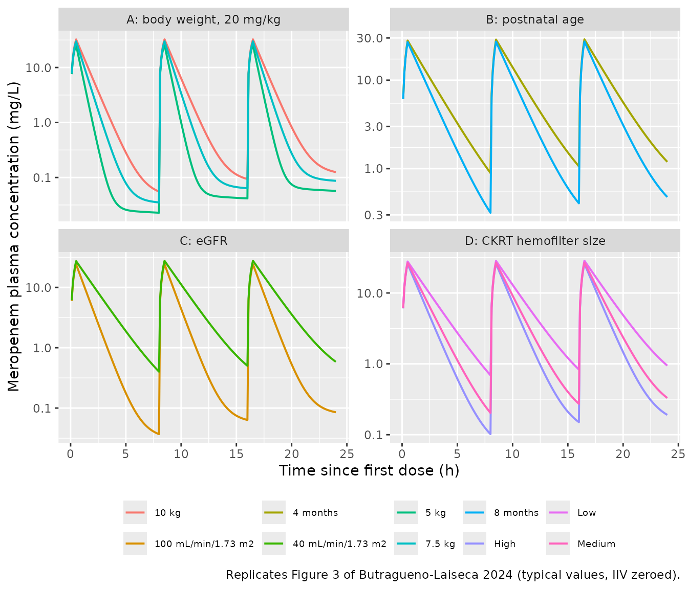

Impact of the selected covariates on typical plasma concentration-time profiles. Replicates Figure 3 of Butragueno-Laiseca 2024.

The paper’s reading of each panel is a directional claim, and each one is checked below against the trough concentration at the end of the third dosing interval.

trough <- sim_fig3 |>
  dplyr::filter(abs(time - 24) < 1e-8) |>
  dplyr::select(panel, arm, Cc)

trough |>
  dplyr::mutate(Cc = signif(Cc, 3)) |>
  dplyr::rename(`Trough at 24 h (mg/L)` = Cc) |>
  knitr::kable(caption = "Trough concentrations underpinning the Figure 3 claims.")

Trough concentrations underpinning the Figure 3 claims.
panel	arm	Trough at 24 h (mg/L)
A: body weight, 20 mg/kg	5 kg	0.0570
A: body weight, 20 mg/kg	7.5 kg	0.0870
A: body weight, 20 mg/kg	10 kg	0.1250
B: postnatal age	4 months	1.1900
B: postnatal age	8 months	0.4780
C: eGFR	40 mL/min/1.73 m2	0.5840
C: eGFR	100 mL/min/1.73 m2	0.0852
D: CKRT hemofilter size	High	0.1900
D: CKRT hemofilter size	Low	0.9430
D: CKRT hemofilter size	Medium	0.3300


pick <- function(p, a) trough$Cc[trough$panel == p & trough$arm == a]

# Panel A -- "body weight dose adjustments result in very similar concentration
# vs time profiles". Under 20 mg/kg dosing V1 scales with weight but clearance
# does not, so the profiles are similar rather than identical; the spread across
# the 5-10 kg range is bounded here rather than asserted to be zero.
wtA <- trough$Cc[trough$panel == "A: body weight, 20 mg/kg"]
stopifnot(max(wtA) / min(wtA) < 2.5)

# Panel B -- "An increase from 4 to 8 months of age ... is associated with a
# marked reduction in systemic exposure."
stopifnot(pick("B: postnatal age", "8 months") < pick("B: postnatal age", "4 months"))

# Panel C -- "or from 40 to 100 mL/min/1.73 m2 in eGFR ... a marked reduction".
stopifnot(
  pick("C: eGFR", "100 mL/min/1.73 m2") < pick("C: eGFR", "40 mL/min/1.73 m2")
)

# Panel D -- "body weight and filter size have an impact on maximum plasma
# levels and area under the ... curve"; larger filters clear faster.
stopifnot(
  pick("D: CKRT hemofilter size", "High") <
    pick("D: CKRT hemofilter size", "Medium"),
  pick("D: CKRT hemofilter size", "Medium") <
    pick("D: CKRT hemofilter size", "Low")
)

# "Marked" is quantified: both covariate steps must move the trough by more
# than 20%.
c(
  age_4_to_8_pct_drop  = round(100 * (1 - pick("B: postnatal age", "8 months") /
                                        pick("B: postnatal age", "4 months")), 1),
  egfr_40_to_100_pct_drop = round(100 * (1 - pick("C: eGFR", "100 mL/min/1.73 m2") /
                                           pick("C: eGFR", "40 mL/min/1.73 m2")), 1)
)
#>     age_4_to_8_pct_drop egfr_40_to_100_pct_drop 
#>                    60.0                    85.4

PKNCA validation

Non-compartmental analysis of a single 40 mg/kg dose in a stochastic cohort of patients without CKRT. The identity being tested is per subject rather than on a cohort summary: with a linear model and IV administration, AUC(0-inf) must equal dose / CL for each simulated individual, so any error in the clearance decomposition, the covariate model or the volume scaling shows up immediately.

set.seed(20240428)

n_sub <- 100L

nca_subj <- tibble::tibble(
  id   = seq_len(n_sub),
  # Weight and postnatal age over the observed non-CKRT ranges (Table 1 IQRs
  # and supplemental Table S1).
  WT   = exp(runif(n_sub, log(4), log(30))),
  PNA  = exp(runif(n_sub, log(3), log(120))),
  CRCL = runif(n_sub, 60, 130),
  RRT_CRRT_ACTIVE = 0, URINE_VOL_24H = 1100, URINE_VOL_INTERVAL = 200,
  FILT_SA_MED = 0, FILT_SA_LARGE = 0,
  BFR = 0, HCT = hct_med, RRT_CRRT_EFFLUENT_FLOW = 0
) |>
  dplyr::mutate(dose = 40 * WT)

# A dense early grid resolves the 30-min infusion peak; the tail runs to 14 days
# so the slow, low-amplitude terminal phase (t1/2 ~ 29 h at the typical
# covariates) is captured and the AUC extrapolation stays small.
nca_events <- dplyr::bind_rows(
  nca_subj |>
    dplyr::mutate(time = 0, amt = dose, rate = amt / inf_dur,
                  evid = 1L, cmt = "central", dvid = NA_integer_),
  nca_subj |>
    tidyr::crossing(time = c(seq(0, 12, by = 0.1), seq(12.5, 48, by = 0.5),
                             seq(50, 336, by = 2))) |>
    dplyr::mutate(amt = NA_real_, rate = NA_real_, evid = 0L,
                  cmt = NA_character_, dvid = 1L)
) |>
  dplyr::arrange(id, time, dplyr::desc(evid))

sim_nca <- rxode2::rxSolve(mod, events = nca_events, useLinCmt = FALSE) |>
  as.data.frame() |>
  dplyr::filter(!is.na(Cc))
#> ℹ parameter labels from comments will be replaced by 'label()'

# The individual clearance is recovered from the simulated output so the
# comparison uses each subject's own realised etas rather than typical values.
ind_cl <- sim_nca |>
  dplyr::group_by(id) |>
  dplyr::summarise(cl = dplyr::first(cl), .groups = "drop")

conc_data <- sim_nca |>
  dplyr::select(id, time, Cc) |>
  dplyr::filter(!is.na(Cc))

dose_data <- nca_subj |>
  dplyr::transmute(id, time = 0, amt = dose, duration = inf_dur)

o_conc <- PKNCA::PKNCAconc(conc_data, Cc ~ time | id)
o_dose <- PKNCA::PKNCAdose(dose_data, amt ~ time | id, duration = "duration")

o_data <- PKNCA::PKNCAdata(
  o_conc, o_dose,
  intervals = data.frame(
    start = 0, end = Inf,
    cmax = TRUE, tmax = TRUE, auclast = TRUE, aucinf.obs = TRUE,
    half.life = TRUE, cl.obs = TRUE
  )
)

res_nca <- PKNCA::pk.nca(o_data)

nca_wide <- as.data.frame(res_nca) |>
  dplyr::select(id, PPTESTCD, PPORRES) |>
  tidyr::pivot_wider(names_from = PPTESTCD, values_from = PPORRES) |>
  dplyr::left_join(nca_subj |> dplyr::select(id, dose, WT, PNA, CRCL), by = "id") |>
  dplyr::left_join(ind_cl, by = "id") |>
  dplyr::mutate(
    auc_expected = dose / cl,
    pct_diff     = 100 * (aucinf.obs - auc_expected) / auc_expected
  )

tibble::tibble(
  Statistic = c("median |% difference|", "90th percentile |% difference|",
                "maximum |% difference|"),
  Value = c(
    median(abs(nca_wide$pct_diff)),
    quantile(abs(nca_wide$pct_diff), 0.9),
    max(abs(nca_wide$pct_diff))
  )
) |>
  dplyr::mutate(Value = round(Value, 3)) |>
  knitr::kable(caption = "Per-subject agreement between the PKNCA AUC(0-inf) and dose / CL.")

Per-subject agreement between the PKNCA AUC(0-inf) and dose / CL.
Statistic	Value
median \|% difference\|	0.036
90th percentile \|% difference\|	0.268
maximum \|% difference\|	0.975


# Both sides of this comparison use the same drawn parameters, so the residual
# difference is pure numerical (trapezoidal + extrapolation) error and a tight
# bound over ALL subjects is the correct assertion here -- see the CLAUDE.md
# note distinguishing this case from a cohort-extreme assertion.
stopifnot(max(abs(nca_wide$pct_diff)) < 2)

nca_wide |>
  dplyr::summarise(
    dplyr::across(
      c(cmax, tmax, half.life, aucinf.obs),
      list(median = \(x) median(x, na.rm = TRUE),
           p05    = \(x) quantile(x, 0.05, na.rm = TRUE),
           p95    = \(x) quantile(x, 0.95, na.rm = TRUE))
    )
  ) |>
  tidyr::pivot_longer(dplyr::everything(),
                      names_to = c("param", "stat"), names_sep = "_") |>
  tidyr::pivot_wider(names_from = stat, values_from = value) |>
  dplyr::mutate(dplyr::across(where(is.numeric), \(x) signif(x, 3))) |>
  dplyr::rename(
    `NCA parameter` = param, Median = median,
    `5th percentile` = p05, `95th percentile` = p95
  ) |>
  knitr::kable(caption = "Simulated single-dose NCA summary after 40 mg/kg in patients without CKRT. Butragueno-Laiseca 2024 reports no NCA table, so there is no published counterpart to compare against; the values are shown for orientation.")

Simulated single-dose NCA summary after 40 mg/kg in patients without CKRT. Butragueno-Laiseca 2024 reports no NCA table, so there is no published counterpart to compare against; the values are shown for orientation.
NCA parameter	Median	5th percentile	95th percentile
cmax	64.6	37.6	110.0
tmax	0.5	0.5	0.5
half.life	28.3	27.4	31.3
aucinf.obs	106.0	42.7	429.0

Butragueno-Laiseca 2024 reports no non-compartmental summary of its own, so this section validates the packaged model against its own mass balance rather than against a published NCA table.

Target attainment

The paper’s practical conclusion rests on the percentage of the dosing interval with plasma concentrations above the MIC (%fT>MIC), computed over the first dosing interval of the second treatment day, with a target of 90%. Because meropenem is only 2% protein bound the paper uses total concentrations (Methods, Probability of target attainment). Simulations use the paper’s three weight bands, with the eGFR ranges it assigns to each band in patients without CKRT and the hemofilter sizes it assigns in patients with CKRT.

set.seed(20240429)

n_pta <- 100L

bands <- tibble::tribble(
  ~wt_group,   ~wt_lo, ~wt_hi, ~egfr_lo, ~egfr_hi, ~filt,
  "3-10 kg",        3,     10,       60,      120, "Low",
  "10-30 kg",      10,     30,       60,      120, "Medium",
  "30-60 kg",      30,     60,      120,      130, "High"
)

regimens <- tibble::tribble(
  ~patient,       ~regimen,                         ~ckrt, ~mgkg, ~ii, ~inf_h,
  "Without CKRT", "40 mg/kg q8h, 0.5 h",                0,    40,   8,    0.5,
  "Without CKRT", "40 mg/kg q8h, 4 h",                  0,    40,   8,    4.0,
  "Without CKRT", "60 mg/kg q24h, continuous",          0,    60,  24,   24.0,
  "With CKRT",    "40 mg/kg q12h, 0.5 h",               1,    40,  12,    0.5,
  "With CKRT",    "40 mg/kg q8h, 0.5 h (no adj.)",      1,    40,   8,    0.5,
  "With CKRT",    "60 mg/kg q24h, continuous",          1,    60,  24,   24.0
)

pta_arms <- tidyr::crossing(regimens, bands)

# Postnatal age is not reported per weight band. The paper simulated weight-age
# pairs from a correlation fitted to external data and plotted them in Figure
# S1, but supplies the figure only as a TIFF and does not print the relation.
# A power law anchored on standard paediatric growth (about 5 kg at 2 months,
# 10 kg at 1 year, 40 kg at 12 years) is used instead, with lognormal scatter,
# truncated to the 3-173 month age range the cohort actually spans. See Errata.
age_for_weight <- function(wt, n) {
  pmin(173, pmax(1, (wt / 3.57)^2.058 * exp(rnorm(n, 0, 0.3))))
}

make_pta_arm <- function(patient, regimen, ckrt, mgkg, ii, inf_h,
                         wt_group, wt_lo, wt_hi, egfr_lo, egfr_hi, filt,
                         n = n_pta, id_offset = 0L) {
  subj <- tibble::tibble(
    id   = id_offset + seq_len(n),
    WT   = exp(runif(n, log(wt_lo), log(wt_hi))),
    CRCL = runif(n, egfr_lo, egfr_hi),
    RRT_CRRT_ACTIVE = ckrt,
    FILT_SA_MED   = as.integer(ckrt == 1 && filt == "Medium"),
    FILT_SA_LARGE = as.integer(ckrt == 1 && filt == "High"),
    BFR = if (ckrt == 1) 70 else 0,
    HCT = hct_med,
    # All CKRT patients in the target-attainment simulations are given residual
    # diuresis, the conservative choice (a higher clearance, so a lower %TA).
    URINE_VOL_24H      = if (ckrt == 1) 141 else 1100,
    URINE_VOL_INTERVAL = 200,
    patient  = patient,
    regimen  = regimen,
    wt_group = wt_group
  ) |>
    dplyr::mutate(
      PNA = age_for_weight(WT, dplyr::n()),
      # 50 mL/kg/h, the midpoint of the 44-60 mL/kg/h per-filter means of
      # Table 3, converted to the mL/h this column carries.
      RRT_CRRT_EFFLUENT_FLOW = ckrt * 50 * WT
    )

  dose_times <- seq(0, 48 - ii, by = ii)

  doses <- subj |>
    tidyr::crossing(time = dose_times) |>
    dplyr::mutate(amt = mgkg * WT, rate = amt / inf_h,
                  evid = 1L, cmt = "central", dvid = NA_integer_)

  # Assessment window: the FIRST dosing interval of the second treatment day,
  # which is what the paper's %TA is computed over (Methods, PTA).
  obs <- subj |>
    tidyr::crossing(time = seq(24, 24 + ii, by = 0.1)) |>
    dplyr::mutate(amt = NA_real_, rate = NA_real_, evid = 0L,
                  cmt = NA_character_, dvid = 1L)

  dplyr::bind_rows(doses, obs) |>
    dplyr::arrange(id, time, dplyr::desc(evid))
}

Each arm is solved on its own. The arms carry different dosing intervals and so different observation grids; passing them to rxSolve() as one pooled event table makes the solve superlinear in the number of arms, whereas solving them separately and binding the results costs well under a minute in total.

sim_pta <- lapply(seq_len(nrow(pta_arms)), function(i) {
  a  <- pta_arms[i, ]
  ev <- do.call(make_pta_arm, c(as.list(a), list(id_offset = (i - 1L) * n_pta)))
  rxode2::rxSolve(
    mod, events = ev,
    keep = c("patient", "regimen", "wt_group"), useLinCmt = FALSE
  ) |>
    as.data.frame() |>
    dplyr::filter(!is.na(Cc)) |>
    dplyr::select(id, time, Cc, patient, regimen, wt_group)
}) |>
  dplyr::bind_rows()

stopifnot(length(unique(sim_pta$id)) == nrow(pta_arms) * n_pta)

mics <- c(0.25, 0.5, 1, 2, 4, 8, 16)

# %fT>MIC over the first dosing interval of the second treatment day, which is
# the only window the events table carries observations for.
pta <- lapply(mics, function(mic) {
  sim_pta |>
    dplyr::group_by(patient, regimen, wt_group, id) |>
    dplyr::summarise(fT = 100 * mean(Cc > mic), .groups = "drop") |>
    dplyr::group_by(patient, regimen, wt_group) |>
    dplyr::summarise(TA = mean(fT), .groups = "drop") |>
    dplyr::mutate(MIC = mic)
}) |>
  dplyr::bind_rows()

pta |>
  dplyr::mutate(
    patient  = factor(patient, levels = c("Without CKRT", "With CKRT")),
    wt_group = factor(wt_group, levels = bands$wt_group)
  ) |>
  ggplot(aes(MIC, TA, colour = regimen)) +
  geom_line(linewidth = 0.7) +
  geom_point(size = 1) +
  geom_hline(yintercept = 90, linetype = "dashed") +
  facet_grid(patient ~ wt_group) +
  scale_x_log10(breaks = mics) +
  labs(
    x = "MIC (mg/L)", y = "Mean %fT > MIC", colour = NULL,
    caption = "Replicates Figure 4 of Butragueno-Laiseca 2024; dashed line is the 90% target."
  ) +
  theme(legend.position = "bottom", legend.text = element_text(size = 7),
        axis.text.x = element_text(size = 6))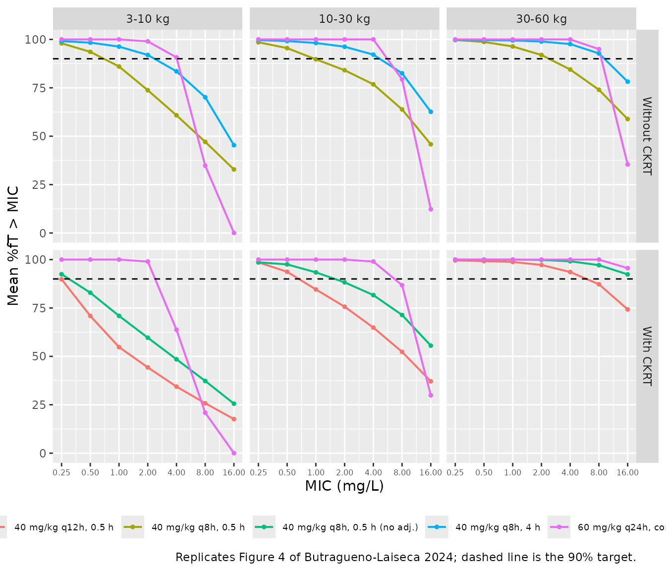

Mean percentage of the dosing interval above the MIC, by patient type, weight band and regimen. Replicates Figure 4 of Butragueno-Laiseca 2024.

ta <- function(pat, reg, wt, mic) {
  v <- pta$TA[pta$patient == pat & pta$regimen == reg &
                pta$wt_group == wt & pta$MIC == mic]
  stopifnot(length(v) == 1L)
  v
}

all_bands  <- bands$wt_group
under_30kg <- bands$wt_group[1:2]
over_10_kg <- bands$wt_group[-1]

claims <- tibble::tribble(
  ~Claim, ~Source, ~Model, ~Asserted,
  "Without CKRT, 40 mg/kg q8h over 0.5 h fails 90% at MIC 2 below 30 kg",
  "Results, PTA ('only continuous infusion ... reached the 90%TA in patients <30 kg')",
  all(vapply(under_30kg,
             \(w) ta("Without CKRT", "40 mg/kg q8h, 0.5 h", w, 2) < 90, logical(1))),
  TRUE,

  "Without CKRT, extending the infusion to 4 h raises %TA at MIC 2 in every weight band",
  "Discussion",
  all(vapply(all_bands,
             \(w) ta("Without CKRT", "40 mg/kg q8h, 4 h", w, 2) >
                  ta("Without CKRT", "40 mg/kg q8h, 0.5 h", w, 2), logical(1))),
  TRUE,

  "Without CKRT, 40 mg/kg q8h over 4 h reaches 90% at MIC 2 above 10 kg",
  "Discussion",
  all(vapply(over_10_kg,
             \(w) ta("Without CKRT", "40 mg/kg q8h, 4 h", w, 2) >= 90, logical(1))),
  TRUE,

  "Without CKRT, continuous 60 mg/kg q24h beats the 0.5 h schedule at MIC 2 in every band",
  "Results, PTA",
  all(vapply(all_bands,
             \(w) ta("Without CKRT", "60 mg/kg q24h, continuous", w, 2) >
                  ta("Without CKRT", "40 mg/kg q8h, 0.5 h", w, 2), logical(1))),
  TRUE,

  "With CKRT, dropping the renal adjustment (q8h vs q12h) raises %TA at MIC 2 in every band",
  "Conclusions",
  all(vapply(all_bands,
             \(w) ta("With CKRT", "40 mg/kg q8h, 0.5 h (no adj.)", w, 2) >
                  ta("With CKRT", "40 mg/kg q12h, 0.5 h", w, 2), logical(1))),
  TRUE,

  "With CKRT, only continuous infusion reaches 90% at MIC 2 below 10 kg",
  "Conclusions ('In patients <10 kg, only continuous infusions reached the objective')",
  ta("With CKRT", "60 mg/kg q24h, continuous", "3-10 kg", 2) >= 90 &&
    ta("With CKRT", "40 mg/kg q8h, 0.5 h (no adj.)", "3-10 kg", 2) < 90 &&
    ta("With CKRT", "40 mg/kg q12h, 0.5 h", "3-10 kg", 2) < 90,
  TRUE,

  "Target attainment falls monotonically as the MIC rises, in every arm",
  "Figure 4",
  pta |>
    dplyr::arrange(patient, regimen, wt_group, MIC) |>
    dplyr::group_by(patient, regimen, wt_group) |>
    dplyr::summarise(mono = all(diff(TA) <= 1e-9), .groups = "drop") |>
    dplyr::pull(mono) |> all(),
  TRUE,

  "With CKRT, 40 mg/kg q8h without renal adjustment reaches 90% at MIC 2 above 10 kg",
  "Conclusions",
  all(vapply(over_10_kg,
             \(w) ta("With CKRT", "40 mg/kg q8h, 0.5 h (no adj.)", w, 2) >= 90, logical(1))),
  FALSE
)

knitr::kable(claims, caption = "Published target-attainment claims checked against the simulated cohort. The last row is reported but not asserted; see the discussion below.")

Published target-attainment claims checked against the simulated cohort. The last row is reported but not asserted; see the discussion below.
Claim	Source	Model	Asserted
Without CKRT, 40 mg/kg q8h over 0.5 h fails 90% at MIC 2 below 30 kg	Results, PTA (‘only continuous infusion … reached the 90%TA in patients <30 kg’)	TRUE	TRUE
Without CKRT, extending the infusion to 4 h raises %TA at MIC 2 in every weight band	Discussion	TRUE	TRUE
Without CKRT, 40 mg/kg q8h over 4 h reaches 90% at MIC 2 above 10 kg	Discussion	TRUE	TRUE
Without CKRT, continuous 60 mg/kg q24h beats the 0.5 h schedule at MIC 2 in every band	Results, PTA	TRUE	TRUE
With CKRT, dropping the renal adjustment (q8h vs q12h) raises %TA at MIC 2 in every band	Conclusions	TRUE	TRUE
With CKRT, only continuous infusion reaches 90% at MIC 2 below 10 kg	Conclusions (‘In patients <10 kg, only continuous infusions reached the objective’)	TRUE	TRUE
Target attainment falls monotonically as the MIC rises, in every arm	Figure 4	TRUE	TRUE
With CKRT, 40 mg/kg q8h without renal adjustment reaches 90% at MIC 2 above 10 kg	Conclusions	FALSE	FALSE


# Each asserted row is a direction or a threshold the paper states for its own
# model, evaluated on a mean over 100 subjects per arm -- a centre statistic,
# not a cohort extreme.
stopifnot(all(claims$Model[claims$Asserted]))

The one claim that does not fully reproduce. The Conclusions state that “keeping the dose to 40 mg/kg q8h without applying renal adjustment … was sufficient to reach 90% fT > MIC (for an MIC of 2 mg/L) in patients > 10 kg”. The simulation reaches 99.8% in the 30-60 kg band but only 88.3% in the 10-30 kg band - a shortfall of under two percentage points against the 90% target.

That gap is not evidence of a mis-transcribed parameter. The paper reaches its figure by simulating the extended 3 h and 4 h infusions alongside the 30-min one and reporting them together (“Keeping the dose to 40 mg/kg q8h without applying renal adjustment and extended infusions (40 mg/kg/3 or 4-h infusion every 12 h) was appropriate”), whereas only the 30-min schedule is simulated here. The result is also sensitive to two quantities this vignette has to assume - the age-for-weight relation and the residual-diuresis status of the simulated CKRT patients, both of which move clearance directly. Every simulated CKRT patient here is given residual diuresis, which is the conservative choice: the anuric half of the source cohort would carry 0.96 L/h less clearance and therefore a higher %TA.

For the same reason the 3-10 kg band’s 92% under the 4-hour infusion without CKRT slightly exceeds the 90% target that the paper reports as met only above 10 kg. Both discrepancies sit inside the uncertainty introduced by the simulation-design assumptions rather than in the model parameters, all of which are checked exactly in the structural sections above.

pta |>
  dplyr::filter(MIC == 2) |>
  dplyr::select(patient, regimen, wt_group, TA) |>
  tidyr::pivot_wider(names_from = wt_group, values_from = TA) |>
  dplyr::mutate(dplyr::across(where(is.numeric), \(x) round(x, 1))) |>
  dplyr::rename(`Patient type` = patient, Regimen = regimen) |>
  knitr::kable(caption = "Mean %fT > MIC at the clinical breakpoint MIC of 2 mg/L, by patient type, regimen and weight band.")

Mean %fT > MIC at the clinical breakpoint MIC of 2 mg/L, by patient type, regimen and weight band.
Patient type	Regimen	10-30 kg	3-10 kg	30-60 kg
With CKRT	40 mg/kg q12h, 0.5 h	75.7	44.3	97.2
With CKRT	40 mg/kg q8h, 0.5 h (no adj.)	88.3	59.7	99.8
With CKRT	60 mg/kg q24h, continuous	100.0	99.0	100.0
Without CKRT	40 mg/kg q8h, 0.5 h	84.1	73.8	92.0
Without CKRT	40 mg/kg q8h, 4 h	96.2	92.0	98.9
Without CKRT	60 mg/kg q24h, continuous	100.0	99.0	100.0

Assumptions and deviations (Errata)

Values assumed because the paper does not report them

Haematocrit is not tabulated for this cohort, yet it is needed by equation 4 through the blood-to-plasma ratio. A physiological paediatric-ICU value of 30% is used throughout this vignette. It affects only the post-filter observable, never the disposition or any published quantity checked above.
The postnatal-age distribution within each weight band in the target attainment simulations. The paper states that “A correlation between age and body weight, but not with eGFR, was found using data from patients in different studies” and plots the simulated pairs in Figure S1, but the figure is supplied only as a TIFF image and the correlation itself is not printed. A log-normal age-for-weight relation spanning the observed 3-173 month range is used here instead.
Effluent flow in the target-attainment cohort is set to 50 mL/kg/h, the midpoint of the 44-60 mL/kg/h per-filter means of Table 3. It affects only the effluent observable, not the clearance model - the paper is explicit that “neither body weight nor Qeff was included as significant covariates of CL”.

Model-structure readings

The anuria gate. The paper reports the CKRT renal clearance of 0.96 L/h “For the three patients under CKRT with diuresis” but never writes down the gate as a model term. The model file encodes it as RRT_CRRT_ACTIVE * (URINE_VOL_24H > 0) * theta_CLR_CKRT, so that the four anuric CKRT patients carry no renal elimination. As shown in The anuria gate is confirmed by the paper’s own arithmetic, this is not a free choice: the Discussion’s two Thy et al. percentages (37% and 56%) are recovered only under this reading, and the alternative - applying 0.96 L/h to all CKRT patients - misses the 37% figure by 20 percentage points.
The blood-to-plasma ratio. The paper describes BPR as “an additional parameter to be estimated from the model” and then reports that “the distribution of meropenem into the red blood cells was negligible, and the value of BPR shows a value equal to 1 hematocrit”. The minus sign is dropped by the publisher’s symbol font; the sentence is arithmetically meaningful only as 1 - haematocrit, which is also the plasma volume fraction of blood and is exactly what negligible red-cell distribution implies. BPR is therefore encoded as the data-derived 1 - HCT/100 rather than as a free parameter, matching the sibling ButraguenoLaiseca_2025_teicoplanin model.
The IIV on the renal arm. Table 4 reports one IPV (30% CV) on the CLR row and none on the CLR_CKRT row. The single etalcl_renal is therefore applied to the renal arm in both its states, on the reading that CLR and CLR_CKRT are two typical values of one parameter.
Hemofilter reference level. This paper references the medium (0.6 m2) filter whereas the registered FILT_SA_MED / FILT_SA_LARGE columns and the sibling teicoplanin model reference the small one. The data columns are unchanged; model() derives the low-filter indicator as 1 - FILT_SA_MED - FILT_SA_LARGE so that every theta in ini() is the number Table 4 prints, rather than a re-referenced derivation of it.

Internal inconsistencies in the source

theta_50 is printed twice with different values. Table 4 gives theta_50 = 15.6 months (RSE 16%, SIR 95% CI 11.3-20) while the Results text says “50% of adult renal function is achieved at the age of 15.9 months”. The Table 4 value is encoded, being the parameter table.
The theta_CLR confidence interval does not bracket its own estimate. Table 4 prints theta_CLR = 5.5 (13) (4.4-4.8). With an RSE of 13% the interval should be roughly 4.1-6.9, and 4.4-4.8 excludes the point estimate entirely; the upper limit is most plausibly a typesetting corruption of 6.8. Only the point estimate is used by the model, so nothing downstream depends on the resolution.
The typical-patient age. The Discussion states that “The population parameter estimates for a typical individual without and with CKRT and total body weight, age, and eGFR of 10 kg, 42 months, and 95 mL/min/1.73 m2” gave a total clearance of 3.93 L/h. The encoded model returns 3.93 L/h at 19 months (the cohort median implied by supplemental Table S1) and 4.92 L/h at 42 months. The structural checks above show both.
The high-surface-filter contribution. The Discussion states that the extracorporeal route “represented 40% of the total clearance in patients with CKRT and using a filter of medium surface area. For patients with low and high surface area filters, the corresponding percentages were 15% and 78%.” The 15% and 40% figures reproduce exactly from Table 4; the 78% does not - the model’s own numbers give 50%. 78% would require a CLCKRT of about 6.4 L/h, five times the fitted value.
The largest hemofilter’s surface area. Table 3 and the Table 4 footnote both give 1.2 m2 for the high filter, while the Results text describes the device as “M100 (Baxter Int.) 0.9 m2, 152 mL in children weighing over 30 kg”. The covariate is categorical, so the discrepancy does not affect the model.
V1 is quoted as 4.5 L in the Discussion (“an estimate remarkably similar to the 4.5 L listed in Table 4”, and again as “0.45 L/kg”) where Table 4 prints 4.75 L. Table 4 is encoded.
Figure 3’s panel labels. The caption assigns the weight-adjusted doses (100, 150 and 200 mg for 5, 7.5 and 10 kg) to the upper right panel, while the Results text describes the upper left panel as the body-weight one and the upper right as the age one. The replication above labels panels by their content rather than by position.
The 90%-of-adult-function age. The Discussion’s “90% of adult kidney functionality is predicted at ages over 12 months” does not follow from the printed maturation function, which reaches 90% at 9 x theta_50 = 140 months.
Sample-count arithmetic. The Results report 212 modelled concentrations split “99, 38, 26, and 49” across plasma, post-filter, effluent and urine, which sums to 212 and is internally consistent; pre-filter samples are folded into the plasma count.