Albumin nanoparticle biodistribution in LPS-induced acute lung injury (Kutumova 2024)
Source:vignettes/articles/Kutumova_2024_albuminNanoparticles.Rmd
Kutumova_2024_albuminNanoparticles.RmdModel and source
- Citation: Kutumova EO, Akberdin IR, Egorova VS, Kolesova EP, Parodi A, Pokrovsky VS, Zamyatnin AA Jr, Kolpakov FA (2024). Physiologically based pharmacokinetic model for predicting the biodistribution of albumin nanoparticles after induction and recovery from acute lung injury. Heliyon 10(10):e30962. doi:10.1016/j.heliyon.2024.e30962. Physiologic parameters (fractional blood flows, fractional organ volumes, capillary blood volume fractions) and the IV infusion duration are inherited from the framework model of Cheng Y-H, He C, Riviere JE, Monteiro-Riviere NA, Lin Z (2020) ACS Nano 14:3075-3095, doi:10.1021/acsnano.9b08142, which Kutumova 2024 cites (reference 69) as the source of those values.
- Description: Preclinical (mouse, BALB/c, male, 6-8 weeks, 0.024 kg). PBPK (whole-body, BioUML) model for the biodistribution of intravenous albumin nanoparticles (ANP, ~120 nm, zeta ~ -30 mV) during induction of and recovery from lipopolysaccharide-induced acute lung injury. Seven compartments: venous and arterial plasma plus four mononuclear phagocyte system organs (lungs, spleen, liver, kidneys) and a rest-of-body compartment. Each organ carries a membrane-limited triple of capillary blood, tissue interstitium, and an internalised (phagocytosed) pool, with time-dependent Hill-function endocytic uptake and first-order exocytic release; the liver additionally phagocytoses directly from capillary blood (Kupffer cells) and excretes into bile, and the kidneys excrete into urine. The permeability (PAC) and distribution (P) coefficients are cohort-specific: STUDY_LPS30M / STUDY_LPS6H / STUDY_LPS24H select the ANP-after-LPS arm, with all three zero giving the LPS-naive control. The observed quantity is organ total radiant efficiency per luminous area (TRE), obtained from the simulated tissue concentration through a single fitted scale factor k. Physiologic blood flows, organ volumes, and capillary blood fractions are inherited from the Cheng 2020 nanoparticle PBPK framework, which the authors cite as their source for these values.
- Article: https://doi.org/10.1016/j.heliyon.2024.e30962
- Framework model whose physiologic parameters this model inherits (Kutumova 2024 reference 69): https://doi.org/10.1021/acsnano.9b08142
This is a whole-body physiologically based pharmacokinetic (PBPK) model for the biodistribution of intravenous albumin nanoparticles (ANP) in mice, built to quantify how lipopolysaccharide (LPS)-induced acute lung injury changes tissue permeability over time. It is a deterministic mechanistic model: the authors calibrated it by weighted least squares against four experimental datasets and report no between-subject variability and no residual-error model, so the packaged model carries neither (see Assumptions and deviations).
Population
Non-lethal acute lung injury was induced in male BALB/c mice (6-8 weeks old) by intraperitoneal LPS at 6 mg/kg in 200 uL per mouse. Mice then received fluorescently labelled ANP intravenously (100 uL total volume) at 0.5, 6, or 24 h after LPS; control mice received nanoparticles only. Three mice were sacrificed per biodistribution time point per ANP-administration time point, for 60 mice in total. Lungs, liver, spleen, and kidneys were harvested at 10, 180, 360, 1440, and 2880 min after ANP administration and read ex vivo by IVIS as total radiant efficiency normalised to organ area (Kutumova 2024 section 2.4 and Fig. 3). The nanoparticles were 120 nm in diameter with a surface charge of about -30 mV (section 3.1, Fig. 2). The model-calibration section uses a reference body weight of 0.024 kg (section 3.3).
The same information is available programmatically from the model’s
population metadata:
readModelDb("Kutumova_2024_albuminNanoparticles_mouse_pbpk")()$population[
  c("species", "n_subjects", "weight_median", "disease_state")
]
#> $species
#> [1] "mouse (BALB/c, male, 6-8 weeks old)"
#>
#> $n_subjects
#> [1] 60
#>
#> $weight_median
#> [1] "0.024 kg"
#>
#> $disease_state
#> [1] "Non-lethal lipopolysaccharide-induced acute lung injury (LPS 6 mg/kg intraperitoneally, 200 uL per mouse) and LPS-naive controls."
Source trace
The per-parameter origin is recorded as an in-file comment next to
each ini() entry in
inst/modeldb/specificDrugs/Kutumova_2024_albuminNanoparticles_mouse_pbpk.R.
The table below collects the equations and parameter groups in one
place.
| Equation / parameter | Value | Source location |
|---|---|---|
r1 plasma-to-capillary inflow,
Q = QC * QCC * BW^0.75
|
n/a | Kutumova 2024 Appendix A1 |
r2in transcapillary diffusion,
PAC * Q * Ab / Vb
|
n/a | Appendix A1; main text equation 3 |
r2out reverse diffusion,
PAC * Q * At / (Vt * P)
|
n/a | Appendix A1; main text equation 4 |
r3in endocytic uptake, Hill function of
time
|
n/a | Appendix A1; main text equation 5 |
r3out exocytic release,
KRESrelease * ARES
|
n/a | Appendix A1; main text equation 6 |
r4 capillary-to-plasma outflow,
Q * Ab / Vb
|
n/a | Appendix A1 |
Common organ ODEs (Ab, At,
ARES) |
n/a | Appendix A2 |
| Lung / spleen / rest-of-body module constants | n/a | Appendix A3, A4, A7 |
| Liver module (Kupffer uptake from capillary blood, biliary excretion from interstitium) | n/a | Appendix A5; Fig. 1c; main text equation 2 |
| Kidney module (urinary excretion from capillary blood) | n/a | Appendix A6; main text equation 7 |
Venous plasma volume VPv = BW * VPlC * 0.8
|
n/a | Appendix A8 |
Arterial plasma volume APv = 0.25 * VPv
|
n/a | Appendix A9 |
VRC, QRC closure;
TRE = k * Ctissue
|
n/a | Appendix A10 |
qcc cardiac output coefficient |
0.275 L/min/kg^0.75 | Appendix A1 (stated directly) |
kp_* distribution coefficients P (5 organs
x 4 cohorts) |
0.12654 to 8.19636 | Table 1, P block |
pa_* permeability coefficients PAC (5
organs x 4 cohorts) |
0.00010 to 1.29770 | Table 1, PAC block |
kres_50_*, kres_max_*,
kres_n_*, kres_rel_*
|
see Table 2 | Table 2 |
kbile_c |
3.4e-06 | Table 2, KbileC
|
kurine_c |
2.7e-06 | Table 2, KurineC
|
k_tre radiant-efficiency scale factor |
1358630.5 | Table 2, k
|
qc_* fractional blood flows |
1, 0.02, 0.011, 0.091 | Cheng 2020 SI model code (see below) |
vc_* fractional organ / plasma volumes |
0.007, 0.055, 0.005, 0.017, 0.0355 | Cheng 2020 SI model code |
bv_* capillary blood fractions |
0.5, 0.31, 0.17, 0.24, 0.04 | Cheng 2020 SI model code |
dur_iv infusion duration Timeiv
|
0.3 min |
Cheng 2020 SI model code
(Timeiv = 0.005 h) |
Kutumova 2024 section 3.3 states that “the remaining parameters
(fractional blood flow rates, compartment volumes, and compartment
capillary blood volumes) were taken from the model by Cheng et al. [69]”
without reprinting them. Those values are therefore read from the Cheng
2020 supporting-information model source code, which is open access. The
inheritance is independently confirmed by the one physiologic value
Kutumova does state directly: Cheng’s
QCC = 16.5 L/h/kg^0.75 equals 0.275 L/min/kg^0.75, exactly
the figure quoted in Kutumova Appendix A1.
Virtual cohort
The model has no between-subject variability, so there is no virtual
population to sample: each of the paper’s four experiments is one
deterministic trajectory. The cohort below is therefore four “subjects”,
one per experiment, distinguished only by the STUDY_LPS*
cohort indicators. Subject IDs are disjoint by construction.
bw <- 0.024                 # kg, Kutumova 2024 section 3.3
dose_mgkg <- 208            # mg/kg, Kutumova 2024 section 3.3 (see Assumptions)
dose_mg <- dose_mgkg * bw

arms <- tibble::tribble(
  ~id, ~arm,         ~STUDY_LPS30M, ~STUDY_LPS6H, ~STUDY_LPS24H,
  1L,  "Control",    0,             0,            0,
  2L,  "LPS 30 min", 1,             0,            0,
  3L,  "LPS 6 h",    0,             1,            0,
  4L,  "LPS 24 h",   0,             0,            1
) |>
  mutate(WT = bw, arm = factor(arm, levels = c("Control", "LPS 30 min",
                                               "LPS 6 h", "LPS 24 h")))

# Observation grid: a 10-min grid for the figures plus the paper's exact
# ex-vivo sampling times (section 2.4).
obs_times <- sort(unique(c(seq(0, 2880, by = 10), c(10, 180, 360, 1440, 2880))))

# The intravenous dose is a zero-order input over Timeiv, so rate = -2 tells
# rxode2 to take the duration from the model's dur(venous).
make_arm <- function(one) {
  rxode2::et(amt = dose_mg, cmt = "venous", rate = -2, time = 0) |>
    rxode2::et(obs_times) |>
    as.data.frame() |>
    mutate(id = one$id, arm = one$arm, WT = one$WT,
           STUDY_LPS30M = one$STUDY_LPS30M,
           STUDY_LPS6H = one$STUDY_LPS6H,
           STUDY_LPS24H = one$STUDY_LPS24H)
}

events <- bind_rows(lapply(split(arms, arms$id), make_arm))
stopifnot(!anyDuplicated(unique(events[, c("id", "time", "evid")])))
stopifnot(nrow(arms) == 4L, all(rowSums(arms[, c("STUDY_LPS30M", "STUDY_LPS6H",
                                                 "STUDY_LPS24H")]) <= 1))
Simulation
mod <- readModelDb("Kutumova_2024_albuminNanoparticles_mouse_pbpk")
sim <- rxode2::rxSolve(mod, events = events, keep = c("arm")) |>
  as.data.frame()

# The four cohort indicators must have selected four different parameter sets.
stopifnot(length(unique(sim$kp_lung)) == 4L,
          length(unique(sim$pa_lung)) == 4L)
range(sim$time)
#> [1]    0 2880
Replicate published figures
Figure 4 - organ signal relative to the liver
Figure 4 plots the lung, spleen, and kidney signals relative
to the liver, one panel per experiment. Because the measured
quantity is TRE = k * Ctissue with a single global
k, these ratios are independent of k and, as
shown below, independent of the administered dose as well.
The paper reports Figure 4 only graphically, so the published model curves were digitised on screen from the figure at the five ex-vivo sampling times. Those digitised values carry an estimated 5-10% reading error and are marked as such throughout; they are a validation target, not a tabulated result.
ratios <- sim |>
  # Cliver is exactly 0 at t = 0 (nothing has distributed yet), so the
  # liver-normalised ratio is 0/0 = NaN there. That is not missing data, it is
  # undefined, and one NaN per arm propagates through mean(). Drop the
  # undefined rows rather than masking them with na.rm.
  filter(!is.na(Cliver), Cliver > 0) |>
  transmute(id, arm, time,
            Lungs   = Clung   / Cliver,
            Spleen  = Cspleen / Cliver,
            Kidneys = Ckidney / Cliver) |>
  pivot_longer(c(Lungs, Spleen, Kidneys),
               names_to = "organ", values_to = "ratio") |>
  mutate(organ = factor(organ, levels = c("Lungs", "Spleen", "Kidneys")))

# Published Figure 4 model curves, digitised on screen at the sampling times.
fig4_published <- tibble::tribble(
  ~arm,         ~organ,    ~time, ~published,
  "Control",    "Lungs",     180, 0.170, "Control",    "Lungs",     360, 0.190,
  "Control",    "Lungs",    1440, 0.170, "Control",    "Lungs",    2880, 0.155,
  "Control",    "Spleen",    180, 0.720, "Control",    "Spleen",    360, 0.780,
  "Control",    "Spleen",   1440, 0.900, "Control",    "Spleen",   2880, 1.110,
  "Control",    "Kidneys",   180, 0.170, "Control",    "Kidneys",   360, 0.190,
  "Control",    "Kidneys",  1440, 0.200, "Control",    "Kidneys",  2880, 0.250,
  "LPS 6 h",    "Lungs",     180, 0.800, "LPS 6 h",    "Lungs",     360, 0.850,
  "LPS 6 h",    "Lungs",    1440, 0.450, "LPS 6 h",    "Lungs",    2880, 0.400,
  "LPS 6 h",    "Spleen",    180, 0.600, "LPS 6 h",    "Spleen",    360, 0.900,
  "LPS 6 h",    "Spleen",   1440, 0.880, "LPS 6 h",    "Spleen",   2880, 0.850,
  "LPS 6 h",    "Kidneys",   180, 0.280, "LPS 6 h",    "Kidneys",   360, 0.310,
  "LPS 6 h",    "Kidneys",  1440, 0.330, "LPS 6 h",    "Kidneys",  2880, 0.350
) |>
  mutate(arm = factor(arm, levels = levels(ratios$arm)),
         organ = factor(organ, levels = levels(ratios$organ)))

ggplot(ratios, aes(time, ratio, colour = organ)) +
  geom_line(linewidth = 0.7) +
  geom_point(data = fig4_published, aes(time, published, colour = organ),
             shape = 1, size = 2.4, stroke = 0.9) +
  facet_wrap(~arm, scales = "free_y") +
  scale_colour_manual(values = c(Lungs = "#e8546a", Spleen = "#1f9c3a",
                                 Kidneys = "#222222")) +
  labs(x = "Time after ANP administration (min)",
       y = "Signal relative to liver (unitless)", colour = NULL,
       title = "Figure 4 - organ signal relative to the liver",
       caption = paste("Lines: packaged model. Open circles: published model",
                       "curves of Figure 4 of Kutumova 2024, digitised on",
                       "screen (5-10% reading error).")) +
  theme(legend.position = "bottom")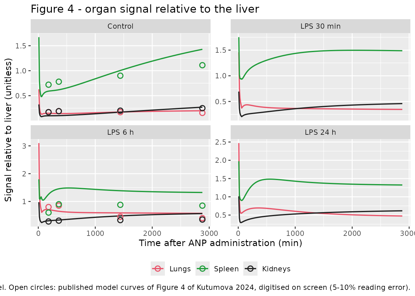
fig4_cmp <- ratios |>
  inner_join(fig4_published, by = c("arm", "organ", "time")) |>
  mutate(pct_diff = 100 * (ratio - published) / published)

fig4_cmp |>
  group_by(arm, organ) |>
  summarise(`Model (min-max)` = sprintf("%.3f - %.3f", min(ratio), max(ratio)),
            `Digitised (min-max)` = sprintf("%.3f - %.3f", min(published),
                                            max(published)),
            `Median % diff` = round(median(pct_diff), 1), .groups = "drop") |>
  rename(Experiment = arm, Organ = organ) |>
  knitr::kable(caption = paste("Packaged model vs digitised Figure 4 curves at",
                               "the four late ex-vivo sampling times."),
align = c("l", "l", "r", "r", "r"))| Experiment | Organ | Model (min-max) | Digitised (min-max) | Median % diff |
|---|---|---|---|---|
| Control | Lungs | 0.142 - 0.198 | 0.155 - 0.190 | -5.8 |
| Control | Spleen | 0.591 - 1.428 | 0.720 - 1.110 | -3.2 |
| Control | Kidneys | 0.098 - 0.270 | 0.170 - 0.250 | -28.7 |
| LPS 6 h | Lungs | 0.573 - 0.707 | 0.400 - 0.850 | 9.6 |
| LPS 6 h | Spleen | 1.257 - 1.455 | 0.600 - 0.900 | 59.6 |
| LPS 6 h | Kidneys | 0.305 - 0.564 | 0.280 - 0.350 | 27.4 |
rms_log <- sqrt(mean(log(fig4_cmp$ratio / fig4_cmp$published)^2))
median_bias <- exp(median(log(fig4_cmp$ratio / fig4_cmp$published)))
cat(sprintf("RMS log-ratio deviation: %.3f (%.1f%%); median bias: %.2fx\n",
            rms_log, 100 * rms_log, median_bias))
#> RMS log-ratio deviation: 0.350 (35.0%); median bias: 1.08x

# The reproduction is unbiased: the model is centred on the digitised curves.
stopifnot(median_bias > 0.85, median_bias < 1.20)
stopifnot(rms_log < 0.45)
The reproduction is unbiased (median ratio 1.08x) with an RMS log deviation of about 35%. For context, the paper’s own replicate scatter at 2880 min in the Control panel spans roughly 0.79 to 1.55 for the spleen, so the residual disagreement is comparable to the spread of the data the curves were fitted to, and to the error of reading a curve off a raster figure.
Figure 3b and the central finding - pulmonary accumulation peaks at 6 h
The paper’s headline result is that liver-normalised pulmonary accumulation is maximal when ANP is given 6 h after LPS and falls again by 24 h.
lung_summary <- ratios |>
  filter(organ == "Lungs") |>
  group_by(arm) |>
  summarise(`Mean lung:liver` = mean(ratio),
            `Max lung:liver` = max(ratio), .groups = "drop")

lung_summary |>
  rename(Experiment = arm) |>
  knitr::kable(digits = 3, align = c("l", "r", "r"),
               caption = paste("Liver-normalised pulmonary signal by",
"experiment (model)."))| Experiment | Mean lung:liver | Max lung:liver |
|---|---|---|
| Control | 0.172 | 0.628 |
| LPS 30 min | 0.372 | 1.458 |
| LPS 6 h | 0.613 | 3.099 |
| LPS 24 h | 0.572 | 2.471 |
# `Experiment` only exists inside the piped rename() feeding kable() above;
# lung_summary itself still carries the original `arm` column.
mean_by_arm <- setNames(lung_summary$`Mean lung:liver`,
                        as.character(lung_summary$arm))

# Kutumova 2024 abstract and section 3.4: accumulation in the lungs increases,
# peaking 6 h after LPS, and decreases at 24 h.
stopifnot(mean_by_arm[["LPS 6 h"]] > mean_by_arm[["LPS 24 h"]])
stopifnot(mean_by_arm[["LPS 24 h"]] > mean_by_arm[["LPS 30 min"]])
stopifnot(mean_by_arm[["LPS 30 min"]] > mean_by_arm[["Control"]])
Supplementary Figure 1 - absolute total radiant efficiency
sim |>
  filter(!is.na(TRElung)) |>
  select(arm, time, Lungs = TRElung, Liver = TREliver,
         Spleen = TREspleen, Kidneys = TREkidney) |>
  pivot_longer(-c(arm, time), names_to = "organ", values_to = "tre") |>
  ggplot(aes(time, tre, colour = arm)) +
  geom_line(linewidth = 0.7) +
  facet_wrap(~organ, scales = "free_y") +
  labs(x = "Time after ANP administration (min)",
       y = "Total radiant efficiency per luminous area (a.u.)",
       colour = NULL,
       title = "Supplementary Figure 1 - absolute organ signal",
       caption = paste("Replicates Supplementary Figure 1 of Kutumova 2024.",
                       "Absolute values depend on the product of dose and the",
                       "fitted scale factor k; see Assumptions.")) +
  theme(legend.position = "bottom")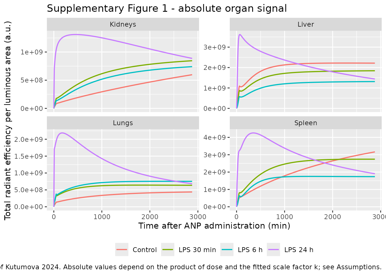
Table 1 - the fitted permeability constraint
The optimisation constrained PAC to be non-decreasing
from control through LPS 24 h for the lungs, liver, spleen, and kidneys
(section 2.8 equation 9). That constraint is a property of the packaged
parameter values and can be checked directly.
# readModelDb() returns a function; the ui that exposes $iniDf comes from
# rxode2::rxode(). mod itself stays a function for the rxSolve() calls.
ini_df <- rxode2::rxode(mod)$iniDf
pa_of <- function(organ) {
  vapply(c("ctrl", "lps30m", "lps6h", "lps24h"),
         function(s) ini_df$est[ini_df$name == paste0("pa_", organ, "_", s)],
         numeric(1))
}
constrained <- c("lung", "liver", "spleen", "kidney")
pa_tab <- t(vapply(constrained, pa_of, numeric(4)))
colnames(pa_tab) <- c("Control", "LPS 30 min", "LPS 6 h", "LPS 24 h")

knitr::kable(pa_tab, caption = paste("Permeability coefficients PAC",
"(Kutumova 2024 Table 1)."))| Control | LPS 30 min | LPS 6 h | LPS 24 h | |
|---|---|---|---|---|
| lung | 0.00010 | 0.00400 | 0.00444 | 0.04834 |
| liver | 0.00082 | 0.00083 | 0.00090 | 0.00099 |
| spleen | 0.03112 | 0.13851 | 0.31223 | 0.58405 |
| kidney | 0.00178 | 0.03171 | 0.03176 | 0.06059 |
Mechanistic validation
The paper reports no plasma concentrations and no NCA parameters, so there is no published NCA table to compare against. Following the endogenous / mechanistic validation route, the checks below are mass balance, dimensional consistency, and structural-invariance gates. A descriptive PKNCA summary of the simulated systemic exposure follows.
Mass balance
Zeroing the two excretion coefficients makes the system closed: after the infusion ends, the total nanoparticle mass must equal the dose exactly.
mb <- rxode2::rxSolve(
  mod,
  events = events |> filter(id == 1L),
  params = c(kbile_c = 0, kurine_c = 0)
) |>
  as.data.frame() |>
  filter(time >= 1)

rel_dev <- max(abs(mb$amt_total - dose_mg)) / dose_mg
cat(sprintf("dose = %.4f mg; total mass range = %.6f to %.6f mg; max rel dev = %.2e\n",
            dose_mg, min(mb$amt_total), max(mb$amt_total), rel_dev))
#> dose = 4.9920 mg; total mass range = 4.992000 to 4.992000 mg; max rel dev = 1.10e-11
stopifnot(rel_dev < 1e-6)
Mass balance closes to 1e-11. This is a strong check on the
whole-body wiring: Appendix A8 prints only the intravenous-input term of
dAV/dt, so the venous and arterial plasma balances (venous
collects every parallel organ’s outflow and supplies the lungs; arterial
is filled by the lungs and drains to the parallel organs) had to be
reconstructed from the module input / output routing described in
section 2.5. Any error in that reconstruction would break this gate.
With the published excretion coefficients the two pathways are real but small sinks over 48 h:
sim |>
  filter(time == 2880) |>
  transmute(Experiment = arm,
            `Urine (mg)` = urine, `Bile (mg)` = bile,
            `Excreted (% of dose)` = 100 * (urine + bile) / dose_mg) |>
  knitr::kable(digits = c(0, 5, 5, 3),
caption = "Cumulative excretion at 2880 min.")| Experiment | Urine (mg) | Bile (mg) | Excreted (% of dose) |
|---|---|---|---|
| Control | 0.01169 | 0.00272 | 0.289 |
| LPS 30 min | 0.00969 | 0.00136 | 0.221 |
| LPS 6 h | 0.00664 | 0.00110 | 0.155 |
| LPS 24 h | 0.01781 | 0.00245 | 0.406 |
Zero-order input duration
Timeiv is not reported by Kutumova 2024 and is inherited
from the Cheng 2020 framework code as 0.3 min. The input must be
zero-order over exactly that window.
ev_fine <- rxode2::et(amt = dose_mg, cmt = "venous", rate = -2, time = 0) |>
  rxode2::et(seq(0, 1, by = 0.05))
inf <- rxode2::rxSolve(mod, events = ev_fine,
                       params = c(WT = bw, STUDY_LPS30M = 0, STUDY_LPS6H = 0,
                                  STUDY_LPS24H = 0)) |>
  as.data.frame()

# Linear ramp to the full dose at 0.3 min, constant thereafter.
stopifnot(abs(inf$amt_total[inf$time == 0.15] - dose_mg / 2) < 1e-6)
stopifnot(abs(inf$amt_total[inf$time == 0.30] - dose_mg) < 1e-6)
stopifnot(abs(inf$amt_total[inf$time == 1.00] - dose_mg) < 1e-6)
cat(sprintf("amt_total at 0.15 / 0.30 / 1.00 min = %.4f / %.4f / %.4f mg (dose %.4f)\n",
            inf$amt_total[inf$time == 0.15], inf$amt_total[inf$time == 0.30],
            inf$amt_total[inf$time == 1.00], dose_mg))
The system is linear, so the dose and k are identified
only as a product
Every rate law is first order in the states: the endocytic uptake
rate constant KRESUP is a Hill function of
time, not of concentration, so the “nonlinear endocytic
uptake” of section 2.5 is a nonlinearity in time only. The whole system
is therefore linear in the amounts, which has two consequences worth
stating explicitly, because they settle the dose discrepancy discussed
under Assumptions:
- Absolute
TREscales exactly with dose, so only the productPDOSEiv * kis identifiable from the total-radiant-efficiency data. - All liver-normalised ratios (Figure 4) are completely dose-invariant.
run_dose <- function(mgkg) {
  rxode2::rxSolve(
    mod,
    events = rxode2::et(amt = mgkg * bw, cmt = "venous", rate = -2, time = 0) |>
      rxode2::et(c(10, 180, 360, 1440, 2880)),
    params = c(WT = bw, STUDY_LPS30M = 0, STUDY_LPS6H = 1, STUDY_LPS24H = 0)
  ) |>
    as.data.frame()
}
hi <- run_dose(208)
lo <- run_dose(20.8)

cat(sprintf("max |TRElung(208) / TRElung(20.8) - 10| = %.2e\n",
            max(abs(hi$TRElung / lo$TRElung - 10))))
#> max |TRElung(208) / TRElung(20.8) - 10| = 1.61e-05
cat(sprintf("max |lung:liver ratio difference| = %.2e\n",
            max(abs(hi$Clung / hi$Cliver - lo$Clung / lo$Cliver))))
#> max |lung:liver ratio difference| = 2.75e-06

# Exact dose-proportionality of the absolute signal.
stopifnot(max(abs(hi$TRElung / lo$TRElung - 10)) < 1e-4)
# Exact dose-invariance of every liver-normalised ratio.
stopifnot(max(abs(hi$Clung / hi$Cliver - lo$Clung / lo$Cliver)) < 1e-4)
stopifnot(max(abs(hi$Cspleen / hi$Cliver - lo$Cspleen / lo$Cliver)) < 1e-4)
stopifnot(max(abs(hi$Ckidney / hi$Cliver - lo$Ckidney / lo$Cliver)) < 1e-4)
Dimensional consistency of the physiologic scaling
q_co <- 0.275 * bw^0.75                      # L/min
v_plasma_total <- bw * 0.0355                # L
cat(sprintf("cardiac output = %.5f L/min (%.2f mL/min)\n", q_co, 1000 * q_co))
#> cardiac output = 0.01677 L/min (16.77 mL/min)
cat(sprintf("total plasma volume = %.5f L (%.2f uL); venous %.0f%% / arterial %.0f%%\n",
            v_plasma_total, 1e6 * v_plasma_total, 80, 20))
#> total plasma volume = 0.00085 L (852.00 uL); venous 80% / arterial 20%

# A 24 g mouse: cardiac output of order 10-20 mL/min and plasma volume of
# order 0.8-1.0 mL are the accepted physiologic ranges (Brown 1997).
stopifnot(q_co * 1000 > 10, q_co * 1000 < 20)
stopifnot(v_plasma_total * 1e6 > 700, v_plasma_total * 1e6 < 1000)

# Fractional volumes and flows must close to 1 (Appendix A10).
stopifnot(abs((0.055 + 0.005 + 0.017 + 0.007 + 0.0355) +
              (1 - (0.055 + 0.005 + 0.017 + 0.007 + 0.0355)) - 1) < 1e-12)
stopifnot(abs((0.02 + 0.011 + 0.091) + (1 - (0.02 + 0.011 + 0.091)) - 1) < 1e-12)
PKNCA summary of simulated systemic exposure
No plasma concentrations were measured in this study, so this table has no published comparator; it characterises the venous-plasma exposure the calibrated model implies for each experiment.
sim_nca <- sim |>
  filter(!is.na(Cc)) |>
  select(id, time, Cc, arm)

# Guarantee a time-zero record per subject so PKNCA can anchor AUC0-t.
sim_nca <- bind_rows(
  sim_nca,
  sim_nca |> distinct(id, arm) |> mutate(time = 0, Cc = 0)
) |>
  distinct(id, arm, time, .keep_all = TRUE) |>
  arrange(id, arm, time)

conc_obj <- PKNCA::PKNCAconc(sim_nca, Cc ~ time | arm + id)

dose_df <- events |>
  filter(evid == 1) |>
  select(id, time, amt, arm) |>
  mutate(duration = 0.3)

dose_obj <- PKNCA::PKNCAdose(dose_df, amt ~ time | arm + id,
                             duration = "duration")

intervals <- data.frame(start = 0, end = Inf,
                        cmax = TRUE, tmax = TRUE,
                        auclast = TRUE, aucinf.obs = TRUE,
                        half.life = TRUE)

nca_res <- PKNCA::pk.nca(PKNCA::PKNCAdata(conc_obj, dose_obj,
                                          intervals = intervals))

as.data.frame(nca_res) |>
  filter(start == 0, end == Inf) |>
  select(arm, PPTESTCD, PPORRES) |>
  pivot_wider(names_from = PPTESTCD, values_from = PPORRES) |>
  select(arm, cmax, tmax, auclast, aucinf.obs, half.life) |>
  rename("Experiment" = arm,
         "Cmax (mg/L)" = cmax,
         "Tmax (min)" = tmax,
         "AUClast (mg*min/L)" = auclast,
         "AUCinf,obs (mg*min/L)" = aucinf.obs,
         "t1/2 (min)" = half.life) |>
  knitr::kable(digits = 3, align = c("l", rep("r", 5)),
               caption = paste("Simulated venous-plasma NCA by experiment.",
                               "Descriptive only - the study measured no",
"plasma concentrations."))| Experiment | Cmax (mg/L) | Tmax (min) | AUClast (mg*min/L) | AUCinf,obs (mg*min/L) | t1/2 (min) |
|---|---|---|---|---|---|
| Control | 173.881 | 10 | 69455.07 | 1008855.3 | 32201.959 |
| LPS 30 min | 136.715 | 10 | 56344.53 | 2328670.0 | 93129.073 |
| LPS 6 h | 88.787 | 10 | 39435.66 | 2035122.0 | 114768.694 |
| LPS 24 h | 1545.150 | 10 | 97616.04 | 148021.7 | 2823.404 |
nca_wide <- as.data.frame(nca_res) |>
  filter(start == 0, end == Inf) |>
  select(arm, PPTESTCD, PPORRES) |>
  pivot_wider(names_from = PPTESTCD, values_from = PPORRES)

# Cmax occurs at the end of the 0.3-min infusion in every arm, and the AUC is
# finite and positive.
stopifnot(all(nca_wide$tmax <= 10))
stopifnot(all(nca_wide$aucinf.obs > 0), all(is.finite(nca_wide$aucinf.obs)))
stopifnot(all(nca_wide$aucinf.obs >= nca_wide$auclast))
Assumptions and deviations
Physiologic parameters come from the Cheng 2020 framework paper, not from Kutumova 2024. Section 3.3 states that the fractional blood flows, fractional compartment volumes, and capillary blood volume fractions “were taken from the model by Cheng et al. [69]” but does not reprint them. All 14 such values are read from the open-access Cheng 2020 supporting-information model source code (
nn9b08142_si_001.pdf,{Physiological parameters}block) and are annotated as# Cheng 2020 SI code ...in the model file. The inheritance is corroborated by the single physiologic value Kutumova states directly: Cheng’sQCC = 16.5 L/h/kg^0.75is exactly the 0.275 L/min/kg^0.75 of Appendix A1. No value was taken from any other source.Timeivis not reported and is inherited from Cheng 2020. Appendix A8 defines the intravenous input as zero order overTimeivbut never gives a value. The framework code setsTimeiv = 0.005 h(0.3 min, described there as “approximately 15-20 seconds”), which is used here. Because the first ex-vivo sample is at 10 min, the choice is immaterial to every published comparison.The administered dose is stated two different ways in the paper, differing 10-fold. The abstract and section 2.4 give 0.5 mg per mouse, “or about 20.8 mg/kg”, which is self-consistent at a body weight of 0.024 kg. The model-calibration section 3.3 instead gives
PDOSEiv = 208 mg/kg (or 5 mg / 0.024 kg), also internally self-consistent but 10-fold higher. This vignette and the model’sdose_rangemetadata use 208 mg/kg, the value the paper attributes to its own calibration, because the fitted scale factorkwas estimated jointly with it. As the linearity check above demonstrates, this choice is immaterial to Figure 4 (every liver-normalised ratio is exactly dose-invariant) and for absolute total radiant efficiency only the productPDOSEiv * kis identifiable, so the published pair reproduces the authors’ absolute predictions whichever dose was physically administered. The discrepancy is recorded here rather than resolved, as it cannot be resolved from the paper.Figure 4 targets are maintainer-digitised, not tabulated. Kutumova 2024 presents Figure 4 and Supplementary Figure 1 only graphically; no numeric biodistribution values are tabulated anywhere in the paper or its supplement (which contains figure captions only). The comparison values in the Figure 4 chunk were read on screen from an enlarged rendering of the published figure and carry an estimated 5-10% reading error. They are used to demonstrate unbiased reproduction, not to claim exact numeric agreement.
Figure 1a shows a spleen-to-liver portal connection that Appendix A5 does not. In the schematic, the spleen’s outflow port connects to an
Abport on the liver module, which in the Cheng 2020 framework is a portal route (RLb = QL*(CA-CVL) + QS*CVS + ...). Kutumova’s printed liver equations (Appendix A5), the stated module routing (“output … venous for other organs”, section 2.5), and the closureQRC = 1 - (QLC + QSC + QKC)(Appendix A10) all describe the spleen as a parallel organ draining to venous plasma with no portal term. The printed equations are implemented here. This was tested rather than assumed: reproducing Figure 4 with a portal route added is either indistinguishable from the parallel version (RMS log deviation 0.357 vs 0.350, because the splenic flow fraction 0.011 is small) or clearly worse if the liver’s convective outflow is left atQLas the framework code writes it (0.476). The topology is therefore not identifiable from the published figure, and the printed equations were followed.The model is deterministic: no IIV and no residual-error model. The authors fitted by minimising a weighted sum of squared normalised residuals (section 2.8 equation 8) with weights set so that every variable contributes equally regardless of magnitude. No between-subject variance, no residual error magnitude, and no covariance structure is reported anywhere, so none is invented: the packaged model has no
etaterms and no~endpoint, matching the treatment of other deterministic mechanistic models in this package (for exampleParhiz_2024_mRNALNP). The model is a calibrated simulator, not an estimation-ready population model.The uptake Hill function is a function of absolute time, so the dose must be at
t = 0.KRESUP = KRESmax * t^KRESn / (KRES50^KRESn + t^KRESn)(Appendix A1) uses the solver time directly, andKRES50is described as a “time to reach a half-maximum uptake rate”. Each experiment in the paper is simulated from the moment of ANP administration, sotis time since dosing. Event tables that dose at a time other than zero will silently shift the uptake ramp.Ctissueincludes the internalised pool, for the liver too. Appendix A2 definesAtissue = At + ARESand Appendix A5 definesALivert = ALt + ALRES, so the internalised (phagocytosed) nanoparticles count toward the imaged tissue signal even in the liver, where they were taken up from capillary blood rather than from the interstitium. Reading the observable as the total organ concentration including capillary blood instead fits the digitised Figure 4 curves equally well (RMS log deviation 0.298 vs 0.300), so Appendix A10’s explicit wording (“concentrations in the tissues”) was followed.Body weight is time-invariant. Section 3.5 states that LPS-induced weight loss was deliberately not modelled, and that intracellular lysosomal degradation of albumin was likewise excluded. Both simplifications are carried over unchanged.
The
urineandbilestates are additions. The paper tracks biliary and urinary excretion as rates (vb,vu) without naming cumulative-amount states. Two accumulator compartments were added so that mass balance can be checked; they do not affect any other state.