mod <- readModelDb("Geers_2022_clozapine")
ui <- rxode2::rxode(mod)
#> ℹ parameter labels from comments will be replaced by 'label()'
Model and source
- Citation: Geers LM, Cohen D, Wehkamp LM, van Wattum HJ, Kosterink JGW, Loonen AJM, Touw DJ. Population pharmacokinetic model and limited sampling strategy for clozapine using plasma and dried blood spot samples. Ther Adv Psychopharmacol. 2022;12:20451253211065857. doi:10.1177/20451253211065857. PMCID: PMC9066631.
- Description: One-compartment population pharmacokinetic model with first-order absorption for oral clozapine in adults with schizophrenia on a stable dose, developed from plasma and dried-blood-spot concentrations by an iterative two-stage Bayesian procedure in MwPharm for Bayesian-forecasting limited-sampling AUC estimation. The volume of distribution scales linearly with body weight; the absorption rate constant is fixed at its literature prior and bioavailability at 1.
- Article: https://doi.org/10.1177/20451253211065857
- Open-access full text: https://www.ncbi.nlm.nih.gov/pmc/articles/PMC9066631/
Geers and colleagues built a small therapeutic-drug-monitoring model
for clozapine with the KinPop module of MwPharm 3.81, using
an iterative two-stage Bayesian procedure rather than nonlinear
mixed-effects modelling. The purpose is a limited sampling strategy
(LSS): one to three concentrations, combined with the population model
by Bayesian forecasting, should recover the steady-state AUC(0-12 h) of
a twice-daily regimen or the AUC(0-24 h) of a once-daily regimen as well
as a full profile would.
The structure is the simplest one the data allowed. A one-compartment
model with first-order absorption won; a lag time, a peripheral
compartment and distribution into fat tissue were each added and
rejected on AIC. Only the elimination rate constant and the per-kg
volume were estimated. The absorption rate constant could not be
estimated (few samples fell in the absorption phase), so it stayed at
the literature prior of the default model (Jerling and colleagues,
1994), and bioavailability was fixed at 1, so the volume is an apparent
V/F.
Concentrations came from two sample types. Venous plasma and
capillary dried-blood-spot (DBS) samples were drawn at the same times,
and each DBS whole-blood result was converted to a plasma-equivalent
concentration with a factor from the authors’ earlier clinical
validation of the method in the same patients. Both were fitted as
plasma, so the model has a single output, Cc, the plasma
clozapine concentration in ug/L.
Population
str(mod()$meta$population)
#> List of 15
#>  $ species       : chr "human"
#>  $ n_subjects    : num 15
#>  $ n_studies     : num 1
#>  $ n_observations: num 121
#>  $ age_range     : chr "18-55 years (inclusion); mean 44, SD 11 years"
#>  $ weight_range  : chr "mean 90 kg, SD 13 kg"
#>  $ height_range  : chr "mean 1.81 m, SD 0.065 m"
#>  $ sex_female_pct: num 20
#>  $ race_ethnicity: chr "Western European descent only (inclusion criterion, to minimise CYP genetic variation)"
#>  $ disease_state : chr "Schizophrenia, outpatients on a stable clozapine dose for at least 2 weeks"
#>  $ dose_range    : chr "Clozapine 75-800 mg/day, mean 287 mg/day; once-daily users split the dose into two halves (evening before and m"| __truncated__
#>  $ regions       : chr "Netherlands (Mental Health Organization Noord-Holland Noord)"
#>  $ renal_function: chr "Serum creatinine mean 80 umol/L, SD 15 umol/L; renal elimination fixed at zero"
#>  $ co_medication : chr "Smokers 10 of 15; plasma-level-affecting co-medication: fluvoxamine 3, omeprazole 3, insulin 1, sodium valproat"| __truncated__
#>  $ notes         : chr "Baseline characteristics from Table 1. Table 1 labels every continuous row 'mean +/- SD' and prints the bounds "| __truncated__
Fifteen adults with schizophrenia (12 men, 3 women) from a Dutch community mental-health organisation, on a stable clozapine dose for at least two weeks, were included. All were of Western European descent, an inclusion criterion meant to limit genetic variation in CYP1A2 expression. Mean age was 44 years and mean body weight 90 kg; doses ranged from 75 to 800 mg/day with a mean of 287 mg/day. Ten of the 15 smoked, and eight carried co-medication that can affect clozapine levels (fluvoxamine, omeprazole, insulin, sodium valproate); none of these was tested as a covariate (Table 1).
To allow daytime sampling, patients on a once-daily regimen took half of their evening dose the evening before sampling and the other half in the morning, so every profile was collected under twice-daily dosing. Samples were taken pre-dose and 2, 4, 6 and 8 h after the morning dose: 49 plasma and 72 DBS concentrations in total (Table 2).
Source trace
| Element | Value | Source location |
|---|---|---|
| Structure: one compartment, first-order absorption, no lag | – | Results, Population PK model; Table 3 (Tlag 0) |
Elimination: Kel = Kelm + Kelr * CLcr,
Kelr set to 0 |
– | Methods, Population PK model |
Volume: per kg body weight, V = Vd * WT
|
– | Methods (‘expressed in L/kg bodyweight’); Results (‘per kg body weight’); Table 3 unit ‘L/kgLBMc’ |
lka |
fixed(log(1.37)) 1/h |
Table 3, Ka 1.37 +/- 0.68 (fixed) |
lkel |
log(0.0641) 1/h |
Table 3, Kelm 0.0641 +/- 0.0365 |
lvd |
log(5.21) L/kg |
Table 3, Vd/F 5.21 +/- 3.82 |
lfdepot |
fixed(log(1)) |
Methods, ‘F of clozapine was fixed at 1’; Table 3 footnote |
etalka |
fixed(0.220230) |
Table 3, SD 0.68 / mean 1.37 = CV 49.6 %,
log(1 + CV^2)
|
etalkel |
0.280840 | Table 3, SD 0.0365 / mean 0.0641 = CV 56.9 %,
log(1 + CV^2)
|
etalvd |
0.430216 | Table 3, SD 3.82 / mean 5.21 = CV 73.3 %,
log(1 + CV^2)
|
addSd |
fixed(10) ug/L |
Methods, assay error ‘SD = 10 + 0.1 x C’ |
propSd |
fixed(0.1) |
Methods, assay error ‘SD = 10 + 0.1 x C’ |
Residual form: linear sum combined1()
|
– | Methods, ‘SD = 10 + 0.1 x C’ |
knitr::kable(
  as.data.frame(ui$iniDf)[, c("name", "est", "fix", "label")],
  digits = 6
)| name | est | fix | label |
|---|---|---|---|
| lka | 0.314811 | TRUE | Absorption rate constant (1/h; literature prior, not estimated) |
| lkel | -2.747311 | FALSE | Elimination rate constant Kelm (1/h) |
| lvd | 1.650580 | FALSE | Apparent volume of distribution per kg body weight Vd/F (L/kg) |
| lfdepot | 0.000000 | TRUE | Oral bioavailability (fraction; F = 1, so V is apparent V/F) |
| addSd | 10.000000 | TRUE | Additive residual SD (ug/L; assay SD intercept, not estimated) |
| propSd | 0.100000 | TRUE | Proportional residual SD (fraction; assay SD slope, not estimated) |
| etalka | 0.220230 | TRUE | Table 3, Ka 1.37 +/- 0.68, held at the literature prior -> 49.6 % CV |
| etalkel | 0.280840 | FALSE | Table 3, Kelm 0.0641 +/- 0.0365 -> 56.9 % CV; shrinkage 0.079 |
| etalvd | 0.430216 | FALSE | Table 3, Vd/F 5.21 +/- 3.82 -> 73.3 % CV; shrinkage 0.054 |
Structural verification
The solved profile matches its own closed form
For a one-compartment model with first-order absorption at steady
state the concentration over a dosing interval tau is
C(t) = F * D * ka / (V * (ka - kel)) * (exp(-kel t) / (1 - exp(-kel tau)) - exp(-ka t) / (1 - exp(-ka tau))).
This chunk solves the representative patient the paper used for its
Monte Carlo simulation (male, 83 kg, 400 mg/day) on both regimens with
zeroRe() and compares the last interval against the closed
form. Both sides use the same typical parameters, so the difference is
pure integrator error and a tight bound is correct.
css_closed <- function(t, dose, tau, ka, kel, v, f = 1) {
  1000 * f * dose / v * ka / (ka - kel) *
    (exp(-kel * t) / (1 - exp(-kel * tau)) - exp(-ka * t) / (1 - exp(-ka * tau)))
}

th <- c(ka = 1.37, kel = 0.0641, vd = 5.21)
wt_rep <- 83
n_days <- 14

typ_events <- function(dose, tau, id) {
  n_dose <- n_days * 24 / tau
  t_last <- (n_dose - 1) * tau
  dplyr::bind_rows(
    data.frame(id = id, time = 0, amt = dose, ii = tau, addl = n_dose - 1, evid = 1L, cmt = "depot"),
    data.frame(id = id, time = t_last + seq(0, tau, by = 0.25), amt = 0, ii = 0, addl = 0, evid = 0L, cmt = "central")
  ) |>
    dplyr::mutate(WT = wt_rep, tau = tau, t_last = t_last)
}
typ_ev <- dplyr::bind_rows(typ_events(200, 12, 1L), typ_events(400, 24, 2L))

typ <- rxode2::rxSolve(
  rxode2::zeroRe(mod), events = typ_ev, keep = c("tau", "t_last"),
  atol = 1e-12, rtol = 1e-12
) |>
  as.data.frame() |>
  dplyr::mutate(
    dose = ifelse(id == 1, 200, 400),
    tad = time - t_last,
    closed = css_closed(tad, dose, tau, th[["ka"]], th[["kel"]], th[["vd"]] * wt_rep),
    rel_err = abs(Cc - closed) / closed
  )
#> ℹ parameter labels from comments will be replaced by 'label()'
#> ℹ omega/sigma items treated as zero: 'etalka', 'etalkel', 'etalvd'
#> Warning: multi-subject simulation without without 'omega'

stopifnot(
  nrow(typ) == 49L + 97L,
  # 14 days is ~20 typical half-lives, so the solve is at steady state to far
  # better than the integrator tolerance.
  max(typ$rel_err) < 1e-6
)

typ |>
  dplyr::group_by(regimen = ifelse(id == 1, "200 mg q12h", "400 mg q24h")) |>
  dplyr::summarise(
    `Cmax (ug/L)` = max(Cc),
    `Tmax (h)` = tad[which.max(Cc)],
    `Ctrough (ug/L)` = Cc[tad == max(tad)],
    `max relative error vs closed form` = format(signif(max(rel_err), 2), scientific = TRUE)
  ) |>
knitr::kable(digits = 2)| regimen | Cmax (ug/L) | Tmax (h) | Ctrough (ug/L) | max relative error vs closed form |
|---|---|---|---|---|
| 200 mg q12h | 764.12 | 1.75 | 418.99 | 9.6e-10 |
| 400 mg q24h | 1025.30 | 2.25 | 265.35 | 2.1e-09 |
The typical clearance of the representative patient is
0.0641 * 5.21 * 83 = 27.7 L/h and the typical half-life
log(2) / 0.0641 = 10.8 h. At 400 mg/day the average
steady-state concentration is about 600 ug/L, inside the 350-700 ug/L
trough window the paper quotes as therapeutic.
ggplot(typ, aes(tad, Cc, colour = ifelse(id == 1, "200 mg q12h", "400 mg q24h"))) +
  geom_line(linewidth = 1) +
  labs(
    x = "Time after dose at steady state (h)", y = "Clozapine plasma concentration (ug/L)",
    colour = NULL,
    title = "Typical steady-state profiles, representative patient (83 kg, 400 mg/day)"
  ) +
  theme_bw()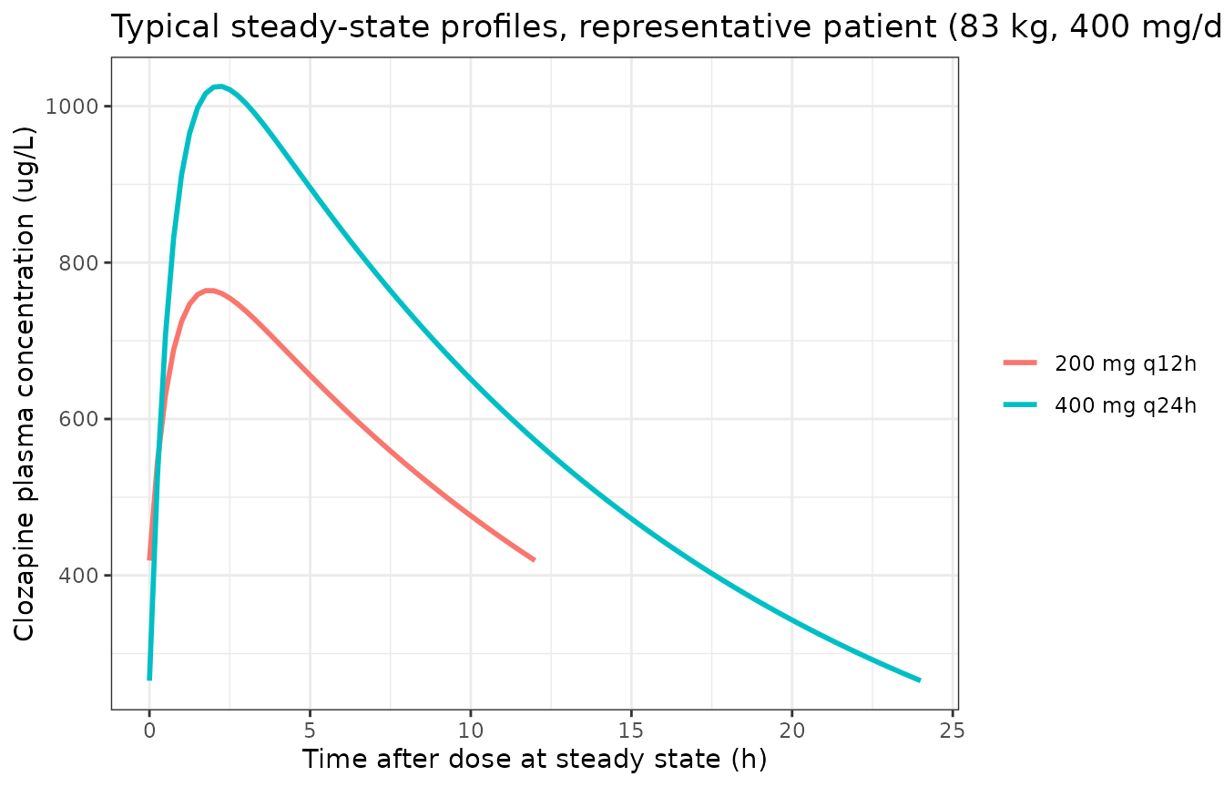
Virtual cohort
The cohort is the source population in outline: body weight drawn around the Table 1 mean of 90 kg (SD 13 kg) and a daily dose of 300 mg, close to the cohort mean of 287 mg/day, given either as 150 mg twice daily or 300 mg once daily. 100 subjects per regimen.
# set.seed() seeds R's RNG, which draws the covariates below, so the COHORT is
# reproducible. It does not seed rxode2's eta sampler, whose streams are
# partitioned per solver thread, so every assertion downstream on an
# eta-driven quantity is written to hold for any draw.
set.seed(20220101)
rxode2::rxSetSeed(20220101)
n_per_arm <- 100L

make_arm <- function(n, dose, tau, id_offset, regimen) {
  wt <- pmin(pmax(rnorm(n, 90, 13), 55), 130)
  n_dose <- n_days * 24 / tau
  t_last <- (n_dose - 1) * tau
  ids <- id_offset + seq_len(n)
  dose_rows <- data.frame(
    id = ids, time = 0, amt = dose, ii = tau, addl = n_dose - 1,
    evid = 1L, cmt = "depot"
  )
  obs_rows <- expand.grid(id = ids, time = t_last + seq(0, tau, by = 0.25)) |>
    dplyr::mutate(amt = 0, ii = 0, addl = 0, evid = 0L, cmt = "central")
  dplyr::bind_rows(dose_rows, obs_rows) |>
    dplyr::left_join(data.frame(id = ids, WT = wt), by = "id") |>
    dplyr::mutate(regimen = regimen, tau = tau, t_last = t_last, dose = dose) |>
    dplyr::arrange(id, time, dplyr::desc(evid))
}

events <- dplyr::bind_rows(
  make_arm(n_per_arm, 150, 12, 0L, "150 mg q12h"),
  make_arm(n_per_arm, 300, 24, n_per_arm, "300 mg q24h")
)
stopifnot(!anyDuplicated(unique(events[, c("id", "time", "evid")])))

events |>
  dplyr::distinct(id, regimen, WT) |>
  dplyr::group_by(regimen) |>
  dplyr::summarise(n = dplyr::n(), `median WT (kg)` = median(WT), `min WT` = min(WT), `max WT` = max(WT)) |>
knitr::kable(digits = 1)| regimen | n | median WT (kg) | min WT | max WT |
|---|---|---|---|---|
| 150 mg q12h | 100 | 92.5 | 59.9 | 122.9 |
| 300 mg q24h | 100 | 91.4 | 57.2 | 112.7 |
Simulation
sim <- rxode2::rxSolve(
  mod, events = events,
  keep = c("regimen", "tau", "t_last", "dose", "WT")
) |>
  as.data.frame() |>
  dplyr::mutate(tad = time - t_last)
#> ℹ parameter labels from comments will be replaced by 'label()'
# The individual parameters ride along in the output; their spread is a check
# that the variances were carried onto the right parameters.
indiv <- sim |> dplyr::distinct(id, regimen, ka, kel, vd, cl, vc)
stopifnot(nrow(indiv) == 2L * n_per_arm)
iiv <- data.frame(
  parameter = c("ka", "kel", "vd"),
  published_mean = c(1.37, 0.0641, 5.21),
  published_cv_pct = 100 * c(0.68 / 1.37, 0.0365 / 0.0641, 3.82 / 5.21),
  simulated_median = c(median(indiv$ka), median(indiv$kel), median(indiv$vd)),
  simulated_cv_pct = 100 * c(sd(indiv$ka) / mean(indiv$ka), sd(indiv$kel) / mean(indiv$kel), sd(indiv$vd) / mean(indiv$vd))
)
knitr::kable(iiv, digits = 3)| parameter | published_mean | published_cv_pct | simulated_median | simulated_cv_pct |
|---|---|---|---|---|
| ka | 1.370 | 49.635 | 1.342 | 48.412 |
| kel | 0.064 | 56.942 | 0.061 | 50.725 |
| vd | 5.210 | 73.321 | 5.454 | 68.362 |
stopifnot(
  # Medians of a 200-subject log-normal draw: generous multiplicative bounds.
  all(abs(log(iiv$simulated_median / iiv$published_mean)) < log(1.35))
)
Simulated concentration-time profiles
Figure 1 of the paper shows the measured concentrations, which span
roughly 30-900 ug/L across the 2-8 h sampling window for the 15 patients
and their range of doses. The shaded band below is the 5th-95th
percentile of the simulated individual concentrations for a 150 mg
twice-daily regimen, with the residual error (sim) shown as
points for a sample of subjects.
vpc <- sim |>
  dplyr::group_by(regimen, tad) |>
  dplyr::summarise(
    p05 = quantile(Cc, 0.05), p50 = median(Cc), p95 = quantile(Cc, 0.95),
    .groups = "drop"
  )

ggplot(vpc, aes(tad, p50)) +
  geom_ribbon(aes(ymin = p05, ymax = p95), alpha = 0.25, fill = "steelblue") +
  geom_line(colour = "steelblue4", linewidth = 1) +
  geom_point(
    data = sim |> dplyr::filter(id %% 10 == 0, tad %in% c(0, 2, 4, 6, 8)),
    aes(tad, sim), inherit.aes = FALSE, alpha = 0.5, size = 1
  ) +
  facet_wrap(~regimen, scales = "free_x") +
  labs(
    x = "Time after dose at steady state (h)", y = "Clozapine plasma concentration (ug/L)",
    title = "Steady-state profiles at 300 mg/day: median and 90% interval"
  ) +
  theme_bw()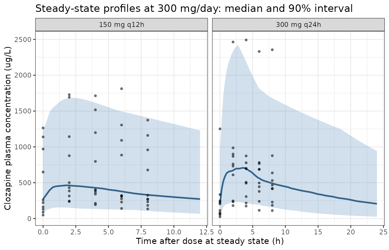
PKNCA validation
Steady-state NCA over the final dosing interval of each regimen. The observation grid places records at both interval endpoints.
sim_nca <- sim |>
  dplyr::filter(!is.na(Cc)) |>
  dplyr::transmute(id, time, Cc, regimen)

# Guarantee a time = 0 record per subject; pre-dose concentration is 0.
sim_nca <- dplyr::bind_rows(
  sim_nca,
  sim_nca |> dplyr::distinct(id, regimen) |> dplyr::mutate(time = 0, Cc = 0)
) |>
  dplyr::distinct(id, regimen, time, .keep_all = TRUE) |>
  dplyr::arrange(id, time)

# Dose records expanded from addl so PKNCA sees every dose.
dose_df <- events |>
  dplyr::filter(evid == 1L) |>
  dplyr::select(id, amt, ii, addl, regimen) |>
  tidyr::uncount(addl + 1L, .id = "k") |>
  dplyr::mutate(time = (k - 1) * ii) |>
  dplyr::select(id, time, amt, regimen)

conc_obj <- PKNCA::PKNCAconc(
  as.data.frame(sim_nca), Cc ~ time | regimen + id,
  concu = "ug/L", timeu = "h"
)
dose_obj <- PKNCA::PKNCAdose(
  as.data.frame(dose_df), amt ~ time | regimen + id,
  doseu = "mg", route = "extravascular"
)

windows <- events |> dplyr::distinct(regimen, tau, t_last)
intervals <- data.frame(
  regimen = windows$regimen,
  start = windows$t_last,
  end = windows$t_last + windows$tau,
  cmax = TRUE, tmax = TRUE, cmin = TRUE, auclast = TRUE, cav = TRUE,
  stringsAsFactors = FALSE
)

nca_res <- PKNCA::pk.nca(PKNCA::PKNCAdata(conc_obj, dose_obj, intervals = intervals))

nca_par <- c("cmax", "tmax", "cmin", "auclast", "cav")
nca_raw <- as.data.frame(nca_res$result) |>
  dplyr::filter(PPTESTCD %in% nca_par)
stopifnot(
  nrow(dplyr::count(nca_raw, regimen, id, PPTESTCD) |> dplyr::filter(n > 1L)) == 0L
)

nca_tbl <- nca_raw |>
  dplyr::select(regimen, id, PPTESTCD, PPORRES) |>
  tidyr::pivot_wider(names_from = PPTESTCD, values_from = PPORRES)
stopifnot(
  nrow(nca_tbl) == 2L * n_per_arm,
  all(vapply(nca_tbl[nca_par], is.numeric, logical(1))),
  !anyNA(nca_tbl$auclast)
)

nca_tbl |>
  dplyr::group_by(regimen) |>
  dplyr::summarise(
    dplyr::across(dplyr::all_of(nca_par), ~ median(.x)),
    .groups = "drop"
  ) |>
  dplyr::rename(
    Regimen = regimen, `Cmax (ug/L)` = cmax, `Tmax (h)` = tmax,
    `Cmin (ug/L)` = cmin, `AUC0-tau (ug*h/L)` = auclast, `Cav (ug/L)` = cav
  ) |>
knitr::kable(digits = 1, caption = "Median steady-state NCA per regimen (300 mg/day).")| Regimen | Cmax (ug/L) | Tmax (h) | Cmin (ug/L) | AUC0-tau (ug*h/L) | Cav (ug/L) |
|---|---|---|---|---|---|
| 150 mg q12h | 471.9 | 1.8 | 272.1 | 4455.2 | 371.3 |
| 300 mg q24h | 727.9 | 2.2 | 205.9 | 9915.0 | 413.1 |
At steady state a linear model must satisfy
CL * AUC(0-tau) = F * Dose, evaluated per subject against
that subject’s own clearance. Both sides use the same drawn parameters;
the gap is trapezoidal error on a 0.25 h grid plus, for a handful of
subjects with very slow elimination, an incomplete approach to steady
state after 14 days. The centre is therefore held tightly and the tail
by a robust quantile.
mb <- nca_tbl |>
  dplyr::left_join(indiv |> dplyr::select(id, cl), by = "id") |>
  dplyr::left_join(events |> dplyr::distinct(id, dose), by = "id") |>
  dplyr::mutate(
    auc_expected = 1000 * dose / cl, # ug*h/L, F = 1
    pct_diff = 100 * (auclast - auc_expected) / auc_expected
  )
stopifnot(
  nrow(mb) == 2L * n_per_arm,
  abs(median(mb$pct_diff)) < 1,
  quantile(abs(mb$pct_diff), 0.9) < 3
)
mb |>
  dplyr::group_by(regimen) |>
  dplyr::summarise(
    `median % diff` = median(pct_diff),
    `90th pct |% diff|` = quantile(abs(pct_diff), 0.9)
  ) |>
knitr::kable(digits = 3, caption = "Simulated AUC0-tau versus F * Dose / CL.")| regimen | median % diff | 90th pct |% diff| |
|---|---|---|
| 150 mg q12h | -0.051 | 0.112 |
| 300 mg q24h | -0.045 | 0.126 |
Comparison against published NCA
The paper reports no NCA summary (Cmax, Tmax, AUC or half-life) for
its cohort, so there is no published NCA table to compare against. The
quantitative results it does report are the limited-sampling performance
statistics of Table 4, which are reproduced in the next section. Figure
2 plots individual full-curve against two-point AUC(0-12 h) values on
axes labelled mg*h/L that run from about 25 to 325; with
the measured concentrations of Figure 1 at 30-900 ug/L, a 12 h AUC can
be at most about 11 mg*h/L, so the Figure 2 axis unit cannot be taken at
face value and that figure is not used as a numeric target.
Reproducing the limited sampling strategy (Table 4)
The paper’s LSS was derived by Monte Carlo simulation of 1000 virtual patients with the characteristics of the representative patient (83 kg, 400 mg/day), followed by Bayesian (maximum a posteriori, MAP) estimation of each patient’s AUC from a subset of sampling times, compared with that patient’s true AUC by the root mean squared prediction error (RMSE, %), the mean prediction error (MPE, %) and r^2. A scheme was “sufficiently predictive” when r^2 > 0.95, RMSE < 15% and MPE < 5%.
The replication below follows that design in plain R so it is
independent of the rxode2 random-number stream: 200 virtual patients
drawn from the model’s IIV (including the Ka prior), steady-state
concentrations from the closed form validated above, assay error
SD = 10 + 0.1 C, and MAP estimation of Kel and
Vd with Ka held at its population value (it
was not Bayesian-estimated in the paper). The true AUC is
F * Dose / CL. The twice-daily interval uses 200 mg every
12 h and the once-daily interval 400 mg every 24 h; the percentage
statistics do not depend on dose.
om <- c(ka = 0.220230, kel = 0.280840, vd = 0.430216)

neg_log_post <- function(eta, obs, times, dose, tau, wt) {
  pred <- css_closed(times, dose, tau, th[["ka"]], th[["kel"]] * exp(eta[1]), th[["vd"]] * exp(eta[2]) * wt)
  sdv <- 10 + 0.1 * pred
  sum(((obs - pred) / sdv)^2 + 2 * log(sdv)) / 2 + sum(eta^2 / om[c("kel", "vd")]) / 2
}

schemes <- data.frame(
  interval = c(rep("0-12", 4), rep("0-24", 4)),
  samples = c("12", "4", "2, 6", "2, 6, 8", "24", "7", "4, 11", "4, 10, 11"),
  pub_rmse = c(23.35, 13.04, 9.06, 6.87, 34.87, 13.58, 7.67, 5.76),
  pub_r2 = c(0.9710, 0.9905, 0.9954, 0.9974, 0.9374, 0.9912, 0.9971, 0.9984),
  pub_mpe = c(5.81, 0.56, -0.20, -0.18, 1.95, -3.02, -0.36, -0.34),
  stringsAsFactors = FALSE
)

set.seed(2022)
n_mc <- 200L
eta_mc <- matrix(rnorm(3 * n_mc), ncol = 3) %*% diag(sqrt(om))
ka_i <- th[["ka"]] * exp(eta_mc[, 1])
kel_i <- th[["kel"]] * exp(eta_mc[, 2])
v_i <- th[["vd"]] * exp(eta_mc[, 3]) * wt_rep

lss_one <- function(interval, samples) {
  tau <- if (interval == "0-12") 12 else 24
  dose <- if (interval == "0-12") 200 else 400
  times <- as.numeric(strsplit(samples, ",")[[1]])
  auc_true <- dose / (kel_i * v_i)
  auc_est <- vapply(seq_len(n_mc), function(i) {
    pred <- css_closed(times, dose, tau, ka_i[i], kel_i[i], v_i[i])
    obs <- pred + rnorm(length(pred)) * (10 + 0.1 * pred)
    fit <- optim(c(0, 0), neg_log_post, obs = obs, times = times, dose = dose, tau = tau, wt = wt_rep)
    dose / (th[["kel"]] * exp(fit$par[1]) * th[["vd"]] * exp(fit$par[2]) * wt_rep)
  }, numeric(1))
  pe <- (auc_est - auc_true) / auc_true
  data.frame(
    sim_rmse = 100 * sqrt(mean(pe^2)),
    sim_r2 = cor(auc_est, auc_true)^2,
    sim_mpe = 100 * mean(pe)
  )
}

lss <- dplyr::bind_cols(
  schemes,
  dplyr::bind_rows(Map(lss_one, schemes$interval, schemes$samples))
)

lss |>
  dplyr::select(interval, samples, pub_rmse, sim_rmse, pub_r2, sim_r2, pub_mpe, sim_mpe) |>
  dplyr::rename(
    `AUC interval (h)` = interval, `Sampling times (h)` = samples,
    `RMSE % (paper)` = pub_rmse, `RMSE % (replication)` = sim_rmse,
    `r2 (paper)` = pub_r2, `r2 (replication)` = sim_r2,
    `MPE % (paper)` = pub_mpe, `MPE % (replication)` = sim_mpe
  ) |>
knitr::kable(digits = c(0, 0, 2, 2, 4, 4, 2, 2), caption = "Replicates Table 4 of Geers 2022.")| AUC interval (h) | Sampling times (h) | RMSE % (paper) | RMSE % (replication) | r2 (paper) | r2 (replication) | MPE % (paper) | MPE % (replication) |
|---|---|---|---|---|---|---|---|
| 0-12 | 12 | 23.35 | 19.56 | 0.9710 | 0.9696 | 5.81 | 1.48 |
| 0-12 | 4 | 13.04 | 14.40 | 0.9905 | 0.9838 | 0.56 | 0.12 |
| 0-12 | 2, 6 | 9.06 | 9.40 | 0.9954 | 0.9918 | -0.20 | -1.41 |
| 0-12 | 2, 6, 8 | 6.87 | 7.55 | 0.9974 | 0.9936 | -0.18 | -0.73 |
| 0-24 | 24 | 34.87 | 36.73 | 0.9374 | 0.9256 | 1.95 | 6.83 |
| 0-24 | 7 | 13.58 | 13.93 | 0.9912 | 0.9708 | -3.02 | -0.78 |
| 0-24 | 4, 11 | 7.67 | 9.26 | 0.9971 | 0.9863 | -0.36 | -1.14 |
| 0-24 | 4, 10, 11 | 5.76 | 7.44 | 0.9984 | 0.9938 | -0.34 | -1.11 |
multi <- lss |> dplyr::filter(grepl(",", samples))
stopifnot(
  # The paper's own acceptance criteria for every two- and three-point scheme,
  # which the replication meets with several points of headroom.
  all(multi$sim_rmse < 15),
  all(multi$sim_r2 > 0.95),
  all(abs(multi$sim_mpe) < 5),
  # Each multi-point RMSE lands within a factor of 1.5 of the published one.
  all(abs(log(multi$sim_rmse / multi$pub_rmse)) < log(1.5))
)
The replication reproduces the paper’s conclusion: the recommended two-point schemes (2 and 6 h for AUC(0-12 h); 4 and 11 h for AUC(0-24 h)) and the three-point schemes meet all three criteria, with RMSE values close to the published ones, and a single trough sample is the weakest predictor. The once-daily trough row in Table 4 is labelled “12 (trough level)”; it is simulated here at 24 h, the trough of a once-daily interval, and lands close to the published RMSE of 34.87% and r^2 of 0.9374 (a 12 h sample in a 24 h interval gives a much smaller error, so the published row cannot be a 12 h sample). Exact agreement is not expected: the paper used 1000 MwPharm Monte Carlo patients and its own MAP implementation.
Assumptions and deviations
Volume normaliser: body weight
Table 3 prints the unit of Vd/F as
L/kgLBMc, the MwPharm fat-corrected lean body mass
LBMc = LBM + (WT - LBM) * fd. The prose states twice that
the volume is per kg body weight (“for simplicity clozapine volume of
distribution is expressed in L/kg bodyweight”, Methods; “distribution
volume per kg body weight (Vd)”, Results), and the paper reports that
adding the “percentage of distribution into fatty tissue” (the
fd factor) did not improve the model. The two statements
agree when fd = 1, for which LBMc = WT. The
model therefore uses V = Vd * WT. The choice has little
effect for the paper’s representative patient (83 kg, 188 cm, whose
MwPharm lean body mass 50 + 0.9 * (188 - 152) = 82.4 kg is
almost his weight). For the cohort-mean man (90 kg, 1.81 m, lean body
mass 76 kg) the alternative fd = 0 reading (volume per kg
lean body mass) would give a volume about 15% smaller, and the gap grows
for heavier, shorter patients.
Interpretation of the reported “mean +/- SD” pairs
MwPharm’s iterative two-stage Bayesian output is a population mean
with an interindividual SD on the natural scale. With parameters assumed
log-normal, the mean is carried as the typical value
(exp(theta)) and the SD converted to a log-scale variance
via omega^2 = log(1 + (SD / mean)^2), as for the other
MwPharm-built model in this library (Daskapan 2019, darunavir). If the
printed value were instead the arithmetic mean of a log-normal, the
median would be lower by the factor sqrt(1 + CV^2) (about
13% for Kel and 19% for Vd). No covariance
between parameters is reported, so the IIV block is diagonal.
Absorption IIV kept as a fixed prior
The absorption rate constant was not Bayesian-estimated; Table 3
lists it with its literature prior SD,
1.37 +/- 0.68 (fixed). The SD is carried as a fixed
variance on etalka so that the full prior the paper used in
Bayesian forecasting is preserved. Set it to zero to reproduce a
typical-absorption model.
Renal elimination omitted
The published elimination model is
Kel = Kelm + Kelr * CLcr with Kelr set to zero
because clozapine is not renally excreted unchanged. With
Kelr = 0 the creatinine-clearance term is identically zero,
so it is not carried and the model needs no creatinine-clearance
column.
DBS conversion
DBS concentrations were converted to plasma-equivalent values before fitting with a conversion factor from the authors’ earlier validation study, which is not restated in this paper. The model predicts plasma concentration; to compare with raw DBS whole-blood measurements the same conversion must be applied.
Covariates not modelled
Smoking, co-medication (notably the CYP1A2 inhibitor fluvoxamine in 3 of 15 patients), sex and age were recorded but not tested as covariates; the paper notes their effect is absorbed into the residual and interindividual variability. The model should not be used to predict the effect of starting or stopping smoking or of interacting drugs.
Once-daily applicability
All profiles were collected on a twice-daily regimen (once-daily users split their dose for the sampling day), so the once-daily AUC(0-24 h) strategy rests on simulation only, as the paper acknowledges.
sessionInfo()
#> R version 4.6.1 (2026-06-24)
#> Platform: x86_64-pc-linux-gnu
#> Running under: Ubuntu 24.04.5 LTS
#>
#> Matrix products: default
#> BLAS:   /usr/lib/x86_64-linux-gnu/openblas-pthread/libblas.so.3
#> LAPACK: /usr/lib/x86_64-linux-gnu/openblas-pthread/libopenblasp-r0.3.26.so;  LAPACK version 3.12.0
#>
#> locale:
#>  [1] LC_CTYPE=C.UTF-8       LC_NUMERIC=C           LC_TIME=C.UTF-8
#>  [4] LC_COLLATE=C.UTF-8     LC_MONETARY=C.UTF-8    LC_MESSAGES=C.UTF-8
#>  [7] LC_PAPER=C.UTF-8       LC_NAME=C              LC_ADDRESS=C
#> [10] LC_TELEPHONE=C         LC_MEASUREMENT=C.UTF-8 LC_IDENTIFICATION=C
#>
#> time zone: UTC
#> tzcode source: system (glibc)
#>
#> attached base packages:
#> [1] stats     graphics  grDevices utils     datasets  methods   base
#>
#> other attached packages:
#> [1] ggplot2_4.0.3         tidyr_1.3.2           dplyr_1.2.1
#> [4] rxode2_5.1.8          PKNCA_0.12.1          nlmixr2lib_0.3.2.9000
#>
#> loaded via a namespace (and not attached):
#>  [1] gtable_0.3.6        xfun_0.61           bslib_0.12.0
#>  [4] rxode2lincmt_0.1.0  lattice_0.22-9      vctrs_0.7.3
#>  [7] tools_4.6.1         generics_0.1.4      parallel_4.6.1
#> [10] tibble_3.3.1        symengine_0.2.14    pkgconfig_2.0.3
#> [13] data.table_1.18.6.1 checkmate_2.3.4     RColorBrewer_1.1-3
#> [16] S7_0.2.2            desc_1.4.3          lifecycle_1.0.5
#> [19] compiler_4.6.1      farver_2.1.2        textshaping_1.0.5
#> [22] fontawesome_0.5.3   htmltools_0.5.9     sys_3.4.3
#> [25] sass_0.4.10         yaml_2.3.12         pillar_1.11.1
#> [28] pkgdown_2.2.1       crayon_1.5.3        jquerylib_0.1.4
#> [31] whisker_0.4.1       openssl_2.4.2       cachem_1.1.0
#> [34] nlme_3.1-169        tidyselect_1.2.1    digest_0.6.39
#> [37] lotri_1.0.5         purrr_1.2.2         labeling_0.4.3
#> [40] rxode2ll_2.0.18     fastmap_1.2.0       grid_4.6.1
#> [43] cli_3.6.6           dparser_1.3.1-14    magrittr_2.0.5
#> [46] withr_3.0.3         scales_1.4.0        backports_1.5.1
#> [49] rmarkdown_2.32      otel_0.2.0          askpass_1.2.1
#> [52] ragg_1.5.2          memoise_2.0.1       evaluate_1.0.5
#> [55] knitr_1.52          rex_1.2.2           PreciseSums_0.7
#> [58] rlang_1.3.0         downlit_0.4.5       Rcpp_1.1.2
#> [61] glue_1.8.1          xml2_1.6.0          jsonlite_2.0.0
#> [64] R6_2.6.1            systemfonts_1.3.2   fs_2.1.0