Fluconazole after fosfluconazole (Tanzawa 2022) • nlmixr2lib

Model and source

Citation: Tanzawa A, Saito J, Shoji K, Kojo Y, Funaki T, Maruyama H, Isayama T, Ito Y, Nakamura H, Yamatani A. Fluconazole Population Pharmacokinetics after Fosfluconazole Administration and Dosing Optimization in Extremely Low-Birth-Weight Infants. Microbiol Spectr. 2022;10(2):e01952-21. doi:10.1128/spectrum.01952-21
Description: One-compartment population PK model for fluconazole formed by first-order conversion of intravenous fosfluconazole (dosed as fluconazole equivalent), with allometric weight scaling and power effects of postmenstrual age, serum creatinine and alkaline phosphatase on clearance, in extremely low-birth-weight infants (Tanzawa 2022)
Article: https://doi.org/10.1128/spectrum.01952-21 (open access, CC BY 4.0)

Fosfluconazole is a phosphate-ester prodrug of fluconazole that alkaline phosphatase converts to fluconazole. Its higher solubility lets the same dose be given in a smaller infusion volume, which matters for infants on strict fluid restriction. Tanzawa 2022 describes serum fluconazole after intravenous fosfluconazole with a one-compartment model and first-order conversion. The prodrug was not measured, so it is carried as an input compartment (depot) that drains into fluconazole (central) at the conversion rate constant kc (ka in the model). Doses are in mg of fluconazole equivalent and go into depot.

mod <- readModelDb("Tanzawa_2022_fluconazole")

Population

Eighteen extremely low-birth-weight infants (birth weight < 1,000 g) with central vascular access received fosfluconazole prophylaxis in the NICU of the National Center for Child Health and Development, Tokyo, between March and August 2020 (Tanzawa 2022 Table 1). Median gestational age was 23.2 weeks (IQR 23.1-26.4), birth weight 748 g (IQR 521-866), and over the study period postmenstrual age (PMA) was 28.5 weeks (IQR 26.3-31.7), current weight 750 g (IQR 580-923), serum creatinine (SCr) 0.64 mg/dL (IQR 0.48-1.07) and alkaline phosphatase (ALP) 958 IU/L (IQR 672-1,208); 61.1% were male. Concomitant amikacin (94.4%), indomethacin (44.4%) and vancomycin (16.7%) were common. Infants received 3 mg/kg fluconazole equivalent every 72 h in weeks 1-2 of life, every 48 h in weeks 3-4 and every 24 h from week 5, with no loading dose, for a median of 17 days. Of 442 scavenged serum samples assayed by LC-MS/MS, 64 below the 0.0031 ug/mL limit of quantitation were excluded; samples were taken a median of 42.2 h (IQR 18.5-61.5) after the latest dose. The model was fitted with Phoenix NLME 8.2. The model was built on a PMA range of 22.9-37.2 weeks and an SCr range of 0.24-2.3 mg/dL; the authors caution against applying it outside those ranges.

The same information is available programmatically:

str(mod()$population)
#> List of 14
#>  $ species       : chr "human"
#>  $ n_subjects    : num 18
#>  $ n_studies     : num 1
#>  $ n_samples     : chr "442 scavenged serum samples assayed; 64 (14.4%) below the 0.0031 ug/mL LLOQ were excluded"
#>  $ age_range     : chr "GA 23.2 weeks (IQR 23.1-26.4); PMA 28.5 weeks (IQR 26.3-31.7) over the study, modelled range 22.9-37.2 weeks; d"| __truncated__
#>  $ weight_range  : chr "Birth weight 748 g (IQR 521-866); current weight 750 g (IQR 580-923)"
#>  $ sex_female_pct: num 38.9
#>  $ race_ethnicity: chr "Japanese (single centre in Tokyo; race not tabulated)"
#>  $ disease_state : chr "Extremely low-birth-weight infants (< 1,000 g) with central vascular access receiving fosfluconazole prophylaxi"| __truncated__
#>  $ dose_range    : chr "Fosfluconazole IV 3 mg/kg as fluconazole equivalent, every 72 h in weeks 1-2 of life, every 48 h in weeks 3-4, "| __truncated__
#>  $ regions       : chr "Japan (National Center for Child Health and Development, Tokyo)"
#>  $ renal_function: chr "Serum creatinine 0.64 mg/dL (IQR 0.48-1.07) over the study; modelled range 0.24-2.3 mg/dL"
#>  $ co_medication : chr "Amikacin 94.4%, indomethacin 44.4%, vancomycin 16.7% (Results)"
#>  $ notes         : chr "Table 1 baseline demographics. Prospective single-centre observational study, March-August 2020, opportunistic "| __truncated__

Source trace

Every ini() value carries an in-file comment pointing to its source in inst/modeldb/specificDrugs/Tanzawa_2022_fluconazole.R. The table collects them.

Equation / parameter	Value	Source location
Structure: one compartment, first-order conversion of fosfluconazole	n/a	Results ‘Population PK model building’; Abstract
`lcl` (CL, L/h/kg^0.75)	log(0.011)	Table 3, final model theta_CL
`lvc` (V, L/kg)	log(0.95)	Table 3, final model theta_V
`lka` (conversion rate kc, 1/h)	fixed(log(0.43))	Table 3, theta_kc (see Assumptions)
`e_wt_cl`	fixed(0.75)	Methods ‘PK analysis’: CL scaled by WT^0.75
`e_wt_vc`	fixed(1.0)	Methods ‘PK analysis’: V scaled by WT^1.0
`e_page_cl`	1.52	Table 3, theta_PMA
`e_creat_cl`	-0.17	Table 3, theta_SCr
`e_alp_cl`	0.10	Table 3, theta_ALP
CL equation	`CL = 0.011 * WT^0.75 * (PMA/29)^1.52 * (SCr/0.64)^-0.17 * (ALP/958)^0.10 * exp(eta_CL)`	Results ‘final PK model’; Table 3 footnote a; Table 2 references
V equation	`V = 0.95 * WT * exp(eta_V)`	Results ‘final PK model’; Table 3 footnote b
`etalcl`	0.07600	Table 3, IIV CL 28.1 CV%, `log(1 + 0.281^2)`
`etalvc`	0.02466	Table 3, IIV V 15.8 CV%, `log(1 + 0.158^2)`
`propSd`	0.14	Table 3, proportional residual 14.0 CV%
`addSd` (ug/mL)	0.068	Table 3, additive residual 0.068 ug/mL

Covariate effects stated in the Discussion

The Discussion quotes three effect sizes. They are deterministic functions of the exponents, so they are checked exactly.

th <- mod()$theta
pma_28_vs_42 <- (28 / 42)^th[["e_page_cl"]]
alp_100_to_2000 <- (2000 / 100)^th[["e_alp_cl"]]
scr_1_to_2 <- (2 / 1)^th[["e_creat_cl"]]

effects <- tibble::tibble(
  Statement = c(
    "CL at PMA 28 weeks vs 42 weeks: 'reduced by 50%'",
    "CL as ALP rises from 100 to 2,000 IU/L: 'increases by only 30%'",
    "CL as SCr rises by 1.0 mg/dL (1.0 to 2.0): 'decreased by 10%'"
  ),
  `Model ratio` = round(c(pma_28_vs_42, alp_100_to_2000, scr_1_to_2), 3)
)
knitr::kable(effects)

Statement	Model ratio
CL at PMA 28 weeks vs 42 weeks: ‘reduced by 50%’	0.540
CL as ALP rises from 100 to 2,000 IU/L: ‘increases by only 30%’	1.349
CL as SCr rises by 1.0 mg/dL (1.0 to 2.0): ‘decreased by 10%’	0.889


stopifnot(
  abs(pma_28_vs_42 - 0.5) < 0.05, # 0.540
  abs(alp_100_to_2000 - 1.3) < 0.06, # 1.349
  abs(scr_1_to_2 - 0.9) < 0.02 # 0.889
)

The 28-versus-42-week ratio is 0.54 (a 46% reduction, which the paper rounds to 50%); the ALP statement gives 1.35 (35%, “only 30%”). The SCr statement holds from 1.0 to 2.0 mg/dL (an 11% fall); from the 0.64 mg/dL reference to 1.64 mg/dL the fall is 15%.

Typical infant at steady state against the closed form

For a typical infant (PMA 29 weeks, SCr 0.64 mg/dL, ALP 958 IU/L, weight 0.75 kg), a 3 mg/kg bolus into the prodrug depot every 72 h has a closed-form steady state. The closed form below uses the Table 3 values typed in directly, not the model file, so a mis-transcribed estimate, exponent or unit in the model shows up as a mismatch.

wt_typ <- 0.75
cl_typ <- 0.011 * wt_typ^0.75 # L/h; all covariate ratios equal 1
v_typ <- 0.95 * wt_typ # L
kc <- 0.43
k <- cl_typ / v_typ
dose <- 3 * wt_typ # mg fluconazole equivalent
tau <- 72
t_obs <- c(0, 1, 2, 4, 8, 12, 24, 36, 48, 60, 72)

closed_form <- dose * kc / (v_typ * (kc - k)) *
  (exp(-k * t_obs) / (1 - exp(-k * tau)) - exp(-kc * t_obs) / (1 - exp(-kc * tau)))

typ_events <- dplyr::bind_rows(
  data.frame(time = 0, evid = 1L, cmt = "depot", amt = dose, ii = tau, ss = 1L),
  data.frame(time = t_obs, evid = 0L, cmt = "central", amt = 0, ii = 0, ss = 0L)
) |>
  dplyr::mutate(id = 1L, WT = wt_typ, PAGE = 29, CREAT = 0.64, ALP = 958)

typ_sim <- rxode2::rxSolve(
  rxode2::zeroRe(mod),
  events = typ_events,
  rtol = 1e-10, atol = 1e-12, ssRtol = 1e-10, ssAtol = 1e-12, maxsteps = 1e6
) |>
  as.data.frame()
#> ℹ parameter labels from comments will be replaced by 'label()'
#> ℹ omega/sigma items treated as zero: 'etalcl', 'etalvc'

knitr::kable(
  data.frame(
    `Time (h)` = t_obs,
    `rxSolve (ug/mL)` = signif(typ_sim$Cc, 5),
    `Closed form (ug/mL)` = signif(closed_form, 5),
    check.names = FALSE
  ),
  caption = "Typical-infant steady state, q72h, 3 mg/kg bolus into the prodrug depot."
)

Typical-infant steady state, q72h, 3 mg/kg bolus into the prodrug depot.
Time (h)	rxSolve (ug/mL)	Closed form (ug/mL)
0	2.2436	2.2436
1	3.3122	3.3122
2	3.9845	3.9845
4	4.6465	4.6465
8	4.8707	4.8707
12	4.7147	4.7147
24	4.0768	4.0768
36	3.5115	3.5115
48	3.0244	3.0244
60	2.6049	2.6049
72	2.2436	2.2436

stopifnot(max(abs(typ_sim$Cc / closed_form - 1)) < 1e-6)

This typical infant has a steady-state trough of 2.24 ug/mL, just above the 2 ug/mL target. Its terminal half-life is 56 h.

Virtual cohorts

The subject-level data are not public. The paper’s Monte Carlo simulations used “demographic and laboratory characteristics simulated from the same distribution as in this study” without stating the distributions, so the cohorts below are reconstructed from Table 1:

PMA is drawn uniformly inside each of the paper’s three PMA groups (23-28, 29-36 and 37-39 weeks).
Weight follows PMA. The reconstruction anchors on the Table 1 median (0.75 kg at 28.5 weeks) and assumes 15 g/kg/day postnatal growth, so WT = 0.75 * exp(0.105 * (PMA - 28.5)) with a 20% log-normal scatter. The dose is weight-based, and CL scales with WT^0.75 while V scales with WT. Concentrations therefore depend on weight only through WT^-0.25 in the elimination rate, and this assumption matters little.
SCr and ALP are log-normal around the Table 1 medians with spreads matched to the IQRs (SCr 0.64 mg/dL, log-SD 0.59, truncated to the modelled 0.24-2.3 mg/dL; ALP 958 IU/L, log-SD 0.43).

# rxSetSeed() fixes rxode2's draws for a given solver thread count only, so a
# machine with a different thread count draws a different cohort. Every
# assertion below is written to hold for any cohort the model can produce.
set.seed(20220310)
rxode2::rxSetSeed(20220310)

n_per_arm <- 200

pma_groups <- tibble::tribble(
  ~pma_group, ~pma_lo, ~pma_hi,
  "<=28", 23, 28,
  "29-36", 29, 36,
  ">=37", 37, 39
)
pma_levels <- pma_groups$pma_group

draw_covariates <- function(n, pma_lo, pma_hi) {
  pma <- stats::runif(n, pma_lo, pma_hi)
  tibble::tibble(
    PAGE = pma,
    WT = 0.75 * exp(0.105 * (pma - 28.5)) * exp(stats::rnorm(n, 0, 0.2)),
    CREAT = pmin(pmax(exp(stats::rnorm(n, log(0.64), 0.59)), 0.24), 2.3),
    ALP = exp(stats::rnorm(n, log(958), 0.43))
  )
}

# One steady-state dosing interval per subject: a 3 mg/kg fosfluconazole
# infusion over 0.5 h (Methods 'Dosing simulations') into the prodrug depot,
# flagged ss = 1 so the solve starts at steady state, then observations of
# fluconazole over one interval tau. Observation rows sit on the ODE state
# `central`; rxode2 returns Cc on those rows.
make_ss_events <- function(cov, tau, obs_times, id_offset) {
  cov <- dplyr::mutate(cov, id = id_offset + dplyr::row_number())
  dose <- cov |>
    dplyr::mutate(
      time = 0, evid = 1L, cmt = "depot", amt = 3 * WT,
      rate = amt / 0.5, ii = tau, ss = 1L
    )
  obs <- tidyr::crossing(cov, time = obs_times) |>
    dplyr::mutate(evid = 0L, cmt = "central", amt = 0, rate = 0, ii = 0, ss = 0L)
  dplyr::bind_rows(dose, obs) |>
    dplyr::arrange(id, time, dplyr::desc(evid))
}

Steady-state Monte Carlo (Table 4)

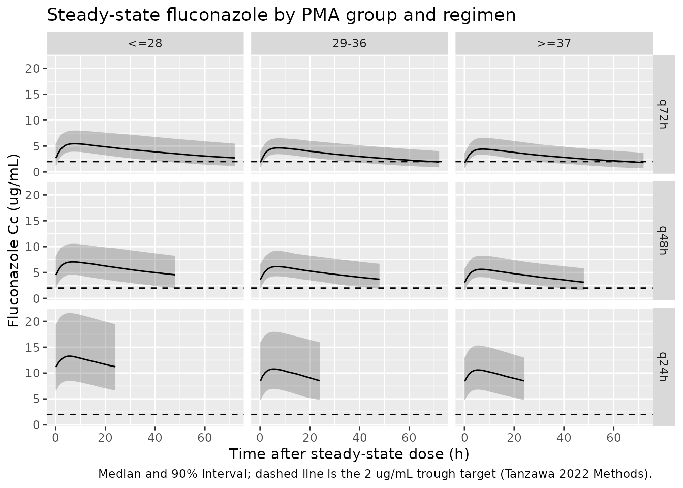
Table 4 of Tanzawa 2022 reports, for each PMA group and three regimens (3 mg/kg every 72, 48 or 24 h), the median and 5th-95th percentiles of the steady-state trough and maximum fluconazole concentrations. It also reports the probability of target attainment (PTA), the share of infants whose trough stays above the 2 ug/mL prophylactic target.

regimens <- tibble::tibble(regimen = c("q72h", "q48h", "q24h"), tau = c(72, 48, 24))
arms <- tidyr::crossing(pma_groups, regimens) |>
  dplyr::mutate(arm = dplyr::row_number())

ss_events <- dplyr::bind_rows(lapply(seq_len(nrow(arms)), function(i) {
  a <- arms[i, ]
  cov <- draw_covariates(n_per_arm, a$pma_lo, a$pma_hi)
  make_ss_events(
    cov,
    tau = a$tau,
    obs_times = c(0, 0.25, 0.5, 0.75, seq(1, a$tau, by = 1)),
    id_offset = (a$arm - 1L) * n_per_arm
  ) |>
    dplyr::mutate(pma_group = a$pma_group, regimen = a$regimen, tau = a$tau)
}))
stopifnot(!anyDuplicated(unique(ss_events[, c("id", "time", "evid")])))

ss_sim <- rxode2::rxSolve(
  mod,
  events = ss_events,
  keep = c("pma_group", "regimen", "tau"),
  maxsteps = 1e6
) |>
  as.data.frame()
#> ℹ parameter labels from comments will be replaced by 'label()'
stopifnot(!anyNA(ss_sim$Cc))

Concentration profiles

ss_sim |>
  dplyr::mutate(
    pma_group = factor(pma_group, levels = pma_levels),
    regimen = factor(regimen, levels = c("q72h", "q48h", "q24h"))
  ) |>
  dplyr::group_by(pma_group, regimen, time) |>
  dplyr::summarise(
    Q05 = stats::quantile(Cc, 0.05), Q50 = stats::median(Cc),
    Q95 = stats::quantile(Cc, 0.95), .groups = "drop"
  ) |>
  ggplot(aes(time, Q50)) +
  geom_ribbon(aes(ymin = Q05, ymax = Q95), alpha = 0.25) +
  geom_line() +
  geom_hline(yintercept = 2, linetype = "dashed") +
  facet_grid(regimen ~ pma_group, scales = "free_x") +
  labs(
    x = "Time after steady-state dose (h)", y = "Fluconazole Cc (ug/mL)",
    title = "Steady-state fluconazole by PMA group and regimen",
    caption = "Median and 90% interval; dashed line is the 2 ug/mL trough target (Tanzawa 2022 Methods)."
  )

PKNCA: steady-state Cmax and trough

ss_conc <- ss_sim |>
  dplyr::filter(!is.na(Cc)) |>
  dplyr::mutate(treatment = paste(regimen, pma_group, sep = " | PMA ")) |>
  dplyr::select(id, time, Cc, treatment, tau)

ss_dose <- ss_events |>
  dplyr::filter(evid == 1) |>
  dplyr::mutate(treatment = paste(regimen, pma_group, sep = " | PMA ")) |>
  dplyr::select(id, time, amt, treatment, tau)

conc_obj <- PKNCA::PKNCAconc(ss_conc, Cc ~ time | treatment + id)
dose_obj <- PKNCA::PKNCAdose(ss_dose, amt ~ time | treatment + id)

# One interval per regimen, opening at the steady-state dose (time 0).
intervals <- ss_dose |>
  dplyr::distinct(treatment, tau) |>
  dplyr::transmute(
    treatment,
    start = 0, end = tau,
    cmax = TRUE, cmin = TRUE, auclast = TRUE
  )

nca_res <- PKNCA::pk.nca(PKNCA::PKNCAdata(conc_obj, dose_obj, intervals = intervals))

At steady state after a slow conversion phase the concentration minimum over the interval is the trough, so PKNCA’s cmin is compared against the Table 4 trough row.

published <- tibble::tribble(
  ~treatment, ~cmin, ~cmax,
  "q72h | PMA <=28", 3.5, 6.6,
  "q72h | PMA 29-36", 2.7, 5.9,
  "q72h | PMA >=37", 2.1, 5.2,
  "q48h | PMA <=28", 5.8, 9.0,
  "q48h | PMA 29-36", 4.7, 7.9,
  "q48h | PMA >=37", 3.7, 6.9,
  "q24h | PMA <=28", 13.7, 16.2,
  "q24h | PMA 29-36", 10.8, 13.9,
  "q24h | PMA >=37", 8.8, 11.9
)

cmp <- nlmixr2lib::ncaComparisonTable(
  simulated = nca_res,
  reference = published,
  by = "treatment",
  params = c("cmax", "cmin"),
  units = c(cmax = "ug/mL", cmin = "ug/mL"),
  tolerance_pct = 20
)
knitr::kable(
  cmp,
  caption = "Median steady-state Cmax and trough: simulated vs Tanzawa 2022 Table 4. * differs by >20%."
)

Median steady-state Cmax and trough: simulated vs Tanzawa 2022 Table 4. * differs by >20%.
NCA parameter	treatment	Reference	Simulated	% diff
Cmax (ug/mL)	q72h \| PMA <=28	6.6	5.46	-17.3%
Cmax (ug/mL)	q72h \| PMA 29-36	5.9	4.65	-21.1%*
Cmax (ug/mL)	q72h \| PMA >=37	5.2	4.42	-15.1%
Cmax (ug/mL)	q48h \| PMA <=28	9	7.04	-21.7%*
Cmax (ug/mL)	q48h \| PMA 29-36	7.9	6.15	-22.1%*
Cmax (ug/mL)	q48h \| PMA >=37	6.9	5.62	-18.6%
Cmax (ug/mL)	q24h \| PMA <=28	16.2	13.3	-18.1%
Cmax (ug/mL)	q24h \| PMA 29-36	13.9	10.8	-22.4%*
Cmax (ug/mL)	q24h \| PMA >=37	11.9	10.6	-11.0%
Cmin (ug/mL)	q72h \| PMA <=28	3.5	2.72	-22.4%*
Cmin (ug/mL)	q72h \| PMA 29-36	2.7	1.92	-28.8%*
Cmin (ug/mL)	q72h \| PMA >=37	2.1	1.82	-13.5%
Cmin (ug/mL)	q48h \| PMA <=28	5.8	4.56	-21.4%*
Cmin (ug/mL)	q48h \| PMA 29-36	4.7	3.7	-21.3%*
Cmin (ug/mL)	q48h \| PMA >=37	3.7	3.13	-15.3%
Cmin (ug/mL)	q24h \| PMA <=28	13.7	11.2	-18.1%
Cmin (ug/mL)	q24h \| PMA 29-36	10.8	8.54	-20.9%*
Cmin (ug/mL)	q24h \| PMA >=37	8.8	8.51	-3.3%

ss_summary <- ss_sim |>
  dplyr::group_by(pma_group, regimen, id) |>
  dplyr::summarise(trough = Cc[time == max(time)], cmax = max(Cc), .groups = "drop") |>
  dplyr::group_by(pma_group, regimen) |>
  dplyr::summarise(
    trough_med = stats::median(trough),
    trough_p05 = stats::quantile(trough, 0.05),
    trough_p95 = stats::quantile(trough, 0.95),
    cmax_med = stats::median(cmax),
    pta = 100 * mean(trough > 2),
    .groups = "drop"
  )

ss_table <- ss_summary |>
  dplyr::mutate(
    pma_group = factor(pma_group, levels = pma_levels),
    regimen = factor(regimen, levels = c("q72h", "q48h", "q24h")),
    `Trough median (5th-95th)` = sprintf("%.1f (%.1f-%.1f)", trough_med, trough_p05, trough_p95),
    `Cmax median` = sprintf("%.1f", cmax_med),
    `PTA (%)` = sprintf("%.1f", pta)
  ) |>
  dplyr::arrange(regimen, pma_group) |>
  dplyr::select(regimen, pma_group, `Trough median (5th-95th)`, `Cmax median`, `PTA (%)`) |>
  dplyr::rename(Regimen = regimen, `PMA group (weeks)` = pma_group)
knitr::kable(
  ss_table,
  caption = paste(
    "Simulated steady-state summaries. Tanzawa 2022 Table 4 q72h troughs:",
    "3.5 (2.2-4.9), 2.7 (1.7-4.0), 2.1 (1.3-3.0) ug/mL; q72h PTA 95.8, 88.9, 43.3%;",
    "q48h and q24h PTA 100% in every group."
  )
)

Simulated steady-state summaries. Tanzawa 2022 Table 4 q72h troughs: 3.5 (2.2-4.9), 2.7 (1.7-4.0), 2.1 (1.3-3.0) ug/mL; q72h PTA 95.8, 88.9, 43.3%; q48h and q24h PTA 100% in every group.
Regimen	PMA group (weeks)	Trough median (5th-95th)	Cmax median	PTA (%)
q72h	<=28	2.7 (1.1-5.5)	5.5	81.0
q72h	29-36	1.9 (0.9-4.0)	4.7	43.5
q72h	>=37	1.8 (0.7-3.7)	4.4	41.5
q48h	<=28	4.6 (2.1-8.2)	7.0	95.5
q48h	29-36	3.7 (1.9-6.7)	6.2	93.0
q48h	>=37	3.1 (1.6-5.8)	5.6	85.5
q24h	<=28	11.2 (6.6-19.4)	13.3	100.0
q24h	29-36	8.5 (4.8-15.9)	10.8	100.0
q24h	>=37	8.5 (4.8-13.0)	10.6	100.0

pct_diff <- ss_summary |>
  dplyr::mutate(treatment = paste(regimen, pma_group, sep = " | PMA ")) |>
  dplyr::inner_join(published, by = "treatment") |>
  dplyr::mutate(
    trough_pct = 100 * (trough_med / cmin - 1),
    cmax_pct = 100 * (cmax_med / cmax - 1)
  )
stopifnot(nrow(pct_diff) == 9L)

# Accumulation between regimens: the q48h / q72h and q24h / q72h median-trough
# ratios within each PMA group. They depend on the elimination rate and on
# nothing else in the cohort, so they test the model against Table 4 without
# the absolute-level offset discussed below.
regimen_ratio <- pct_diff |>
  dplyr::filter(regimen != "q72h") |>
  dplyr::inner_join(
    pct_diff |>
      dplyr::filter(regimen == "q72h") |>
      dplyr::select(pma_group, trough_q72 = trough_med, cmin_q72 = cmin),
    by = "pma_group"
  ) |>
  dplyr::mutate(
    ratio_simulated = trough_med / trough_q72,
    ratio_published = cmin / cmin_q72,
    ratio_pct = 100 * (ratio_simulated / ratio_published - 1)
  )
stopifnot(nrow(regimen_ratio) == 6L)

regimen_ratio |>
  dplyr::transmute(
    `PMA group (weeks)` = pma_group,
    `Trough ratio vs q72h` = regimen,
    Simulated = round(ratio_simulated, 2),
    `Table 4` = round(ratio_published, 2),
    `% diff` = round(ratio_pct, 1)
  ) |>
  knitr::kable(caption = "Accumulation of the median trough relative to q72h, simulated vs Tanzawa 2022 Table 4.")

Accumulation of the median trough relative to q72h, simulated vs Tanzawa 2022 Table 4.
PMA group (weeks)	Trough ratio vs q72h	Simulated	Table 4	% diff
29-36	q24h	4.44	4.00	11.0
29-36	q48h	1.92	1.74	10.6
<=28	q24h	4.13	3.91	5.6
<=28	q48h	1.68	1.66	1.3
>=37	q24h	4.68	4.19	11.8
>=37	q48h	1.73	1.76	-2.0


pta_q72 <- with(dplyr::filter(ss_summary, regimen == "q72h"), stats::setNames(pta, pma_group))

stopifnot(
  # Regimen ratios hold within 20% in every group (realised 1-13%). A wrong
  # CL, V or PMA exponent shifts the elimination rate and moves the q24h ratio
  # by more than that.
  max(abs(regimen_ratio$ratio_pct)) < 20,
  # Daily dosing reaches the target in nearly all infants (Table 4: 100% in
  # every group; realised 100% here).
  all(ss_summary$pta[ss_summary$regimen == "q24h"] > 95),
  # The q72h PTA falls steeply with PMA (Table 4: 95.8 vs 43.3%; realised
  # about 81 vs 42% here, a difference of about 5 binomial SEs above 25).
  pta_q72[["<=28"]] - pta_q72[[">=37"]] > 25
)

Known deviation: absolute level. The simulated median troughs and peaks are lower than Table 4. Across the nine cells the median shortfall is 21% for the trough and 19% for Cmax. The >=37-week cells come closest. The Table 4 values cannot be reached with the published estimates and a cohort resembling Table 1. A q72h trough of 3.5 ug/mL at V = 0.95 L/kg needs an elimination rate of about 0.0091 /h. The final model gives that rate only to an infant of 0.75 kg at a PMA of about 23.6 weeks, at the bottom of the <=28-week group rather than at its centre. The same 20% gap appears in the 29-36-week group. The study-regimen simulation further down sits above the observed concentrations, the opposite direction. So no single misprinted estimate explains the gap, and the model keeps the Table 3 values as printed. The accumulation ratios above, which do not depend on the level, agree.

The Table 4 trough percentiles are also narrower than the reported IIV allows. A 28.1% CV on CL alone spreads the trough wider than Table 4’s 5th-95th interval (2.2-4.9 ug/mL in the <=28-week group). Table 4’s 100% PTA at SCr > 2.0 mg/dL in every PMA group would need almost no between-infant variability. The simulated PTA values below are therefore compared on their trend with SCr, not on their level.

PTA by serum creatinine (Table 4, q72h)

Table 4 also stratifies the q72h PTA by SCr. Each SCr band below is a separate 200-infant arm, with SCr uniform inside the band and the other covariates drawn as above; only the trough is needed.

scr_bands <- tibble::tribble(
  ~scr_band, ~scr_lo, ~scr_hi,
  "<0.5", 0.24, 0.5,
  "0.5-1.0", 0.5, 1.0,
  "1.1-1.5", 1.0, 1.5,
  "1.6-2.0", 1.5, 2.0,
  ">2.0", 2.0, 2.3
)
scr_arms <- tidyr::crossing(pma_groups, scr_bands) |>
  dplyr::mutate(arm = dplyr::row_number())

scr_events <- dplyr::bind_rows(lapply(seq_len(nrow(scr_arms)), function(i) {
  a <- scr_arms[i, ]
  cov <- draw_covariates(n_per_arm, a$pma_lo, a$pma_hi) |>
    dplyr::mutate(CREAT = stats::runif(n_per_arm, a$scr_lo, a$scr_hi))
  make_ss_events(cov, tau = 72, obs_times = 72, id_offset = (a$arm - 1L) * n_per_arm) |>
    dplyr::mutate(pma_group = a$pma_group, scr_band = a$scr_band)
}))
stopifnot(!anyDuplicated(unique(scr_events[, c("id", "time", "evid")])))

scr_sim <- rxode2::rxSolve(
  mod,
  events = scr_events,
  keep = c("pma_group", "scr_band"),
  maxsteps = 1e6
) |>
  as.data.frame()

published_pta <- tibble::tribble(
  ~scr_band, ~`<=28`, ~`29-36`, ~`>=37`,
  "<0.5", 99.2, 50.0, 5.6,
  "0.5-1.0", 100.0, 94.4, 38.9,
  "1.1-1.5", 100.0, 100.0, 77.8,
  "1.6-2.0", 100.0, 100.0, 94.4,
  ">2.0", 100.0, 100.0, 100.0
) |>
  tidyr::pivot_longer(-scr_band, names_to = "pma_group", values_to = "pta_published")

pta_scr <- scr_sim |>
  dplyr::group_by(pma_group, scr_band) |>
  dplyr::summarise(pta_simulated = 100 * mean(Cc > 2), .groups = "drop") |>
  dplyr::inner_join(published_pta, by = c("pma_group", "scr_band")) |>
  dplyr::mutate(
    pma_group = factor(pma_group, levels = pma_levels),
    scr_band = factor(scr_band, levels = scr_bands$scr_band)
  ) |>
  dplyr::arrange(pma_group, scr_band)
stopifnot(nrow(pta_scr) == 15L)

pta_scr |>
  dplyr::mutate(pta_simulated = round(pta_simulated, 1)) |>
  dplyr::rename(
    `PMA group (weeks)` = pma_group, `SCr (mg/dL)` = scr_band,
    `PTA simulated (%)` = pta_simulated, `PTA Table 4 (%)` = pta_published
  ) |>
  knitr::kable(caption = "q72h PTA (trough > 2 ug/mL) by SCr band: simulated vs Tanzawa 2022 Table 4.")

q72h PTA (trough > 2 ug/mL) by SCr band: simulated vs Tanzawa 2022 Table 4.
PMA group (weeks)	SCr (mg/dL)	PTA simulated (%)	PTA Table 4 (%)
<=28	<0.5	61.5	99.2
<=28	0.5-1.0	77.5	100.0
<=28	1.1-1.5	83.0	100.0
<=28	1.6-2.0	87.5	100.0
<=28	>2.0	87.5	100.0
29-36	<0.5	36.5	50.0
29-36	0.5-1.0	56.0	94.4
29-36	1.1-1.5	62.0	100.0
29-36	1.6-2.0	75.5	100.0
29-36	>2.0	76.0	100.0
>=37	<0.5	24.0	5.6
>=37	0.5-1.0	41.5	38.9
>=37	1.1-1.5	61.5	77.8
>=37	1.6-2.0	63.0	94.4
>=37	>2.0	60.5	100.0

pta_lookup <- function(pma, band) {
  v <- pta_scr$pta_simulated[pta_scr$pma_group == pma & pta_scr$scr_band == band]
  if (length(v) != 1L) stop("no unique PTA row for PMA ", pma, ", SCr ", band)
  v
}
stopifnot(
  # Higher SCr lowers CL and raises the trough, so PTA climbs with SCr (Table
  # 4: 5.6 to 100% at >=37 weeks, 50 to 100% at 29-36 weeks). The trend is
  # checked end to end, not band by band. Realised rises of about 35-40 points;
  # with 200 infants per band the binomial SE of a difference is about 5
  # points, so 20 sits about 3 SEs below.
  pta_lookup(">=37", ">2.0") - pta_lookup(">=37", "<0.5") > 20,
  pta_lookup("29-36", ">2.0") - pta_lookup("29-36", "<0.5") > 20,
  # Younger infants clear fluconazole more slowly, so at every SCr band the
  # <=28-week group attains the target more often than the >=37-week group.
  # This is checked on the average over bands, not band by band.
  mean(pta_scr$pta_simulated[pta_scr$pma_group == "<=28"]) -
    mean(pta_scr$pta_simulated[pta_scr$pma_group == ">=37"]) > 15
)

As Table 4 does, the simulation shows PTA climbing with SCr, and the <=28-week group sitting above the >=37-week group. Table 4’s levels near 100% are not reached, for the variability reason given above.

Study regimen and the visual predictive check (Figures 1 and 3)

Figure 3 of Tanzawa 2022 is a VPC of serum fluconazole against time after the latest dose, pooling all regimens. Here 200 virtual infants receive the study regimen from birth: 3 mg/kg every 72 h in weeks 1-2, every 48 h in weeks 3-4 and every 24 h from week 5. Dosing stops at the paper’s median treatment duration of 17 days, so the every-24-h phase is not reached, and is followed by 8 days of washout. Gestational age follows the Table 1 quartiles. PMA advances with postnatal age, and weight grows at 15 g/kg/day from a Table 1-like birth weight. SCr and ALP are held at one draw per infant.

# q72h on days 0-13, then q48h; last dose on day 16 (median duration 17 days).
study_dose_times <- c(seq(0, 312, by = 72), seq(336, 384, by = 48))
end_of_dosing <- 408
obs_grid <- seq(0, end_of_dosing + 192, by = 4)

# Gestational age: piecewise-linear inverse CDF through the Table 1 median and
# IQR (23.2; 23.1-26.4 weeks), with assumed extremes of 22.9 and 27.9 weeks.
ga_quantile <- function(u) stats::approx(c(0, 0.25, 0.5, 0.75, 1), c(22.9, 23.1, 23.2, 26.4, 27.9), xout = u)$y

study_cov <- tibble::tibble(
  id = seq_len(n_per_arm),
  GA = ga_quantile(stats::runif(n_per_arm)),
  BW = pmin(pmax(exp(stats::rnorm(n_per_arm, log(0.748), 0.25)), 0.4), 1.0),
  CREAT = pmin(pmax(exp(stats::rnorm(n_per_arm, log(0.64), 0.59)), 0.24), 2.3),
  ALP = exp(stats::rnorm(n_per_arm, log(958), 0.43))
)

study_events <- tidyr::crossing(study_cov, time = sort(unique(c(study_dose_times, obs_grid)))) |>
  dplyr::mutate(
    PAGE = GA + time / 168,
    WT = BW * exp(0.015 * time / 24)
  )
study_events <- dplyr::bind_rows(
  study_events |>
    dplyr::filter(time %in% study_dose_times) |>
    dplyr::mutate(evid = 1L, cmt = "depot", amt = 3 * WT, rate = amt / 0.5),
  study_events |>
    dplyr::filter(time %in% obs_grid) |>
    dplyr::mutate(evid = 0L, cmt = "central", amt = 0, rate = 0)
) |>
  dplyr::arrange(id, time, dplyr::desc(evid))
stopifnot(!anyDuplicated(unique(study_events[, c("id", "time", "evid")])))

study_sim <- rxode2::rxSolve(mod, events = study_events, maxsteps = 1e6) |>
  as.data.frame() |>
  dplyr::mutate(tad = time - study_dose_times[findInterval(time, study_dose_times)])

# Replicates Figure 3 of Tanzawa 2022: VPC against time after dose (observed
# concentrations include residual error, so the simulated `sim` column is used).
study_sim |>
  dplyr::filter(time > 0) |>
  dplyr::mutate(tad_bin = cut(tad, breaks = c(seq(0, 72, by = 6), 96, 120, 144, 168, 192), include.lowest = TRUE)) |>
  dplyr::group_by(tad_bin) |>
  dplyr::summarise(
    tad = stats::median(tad),
    Q05 = stats::quantile(sim, 0.05), Q50 = stats::median(sim), Q95 = stats::quantile(sim, 0.95),
    .groups = "drop"
  ) |>
  ggplot(aes(tad, Q50)) +
  geom_ribbon(aes(ymin = Q05, ymax = Q95), alpha = 0.25) +
  geom_line() +
  coord_cartesian(xlim = c(0, 200), ylim = c(0, 8)) +
  labs(
    x = "Time after dose (h)", y = "Fluconazole (ug/mL)",
    title = "Study regimen: simulated median and 90% interval",
    caption = "Replicates the layout of Figure 3 of Tanzawa 2022 (observed points 0.5-8 ug/mL, mostly 1-6 ug/mL)."
  )

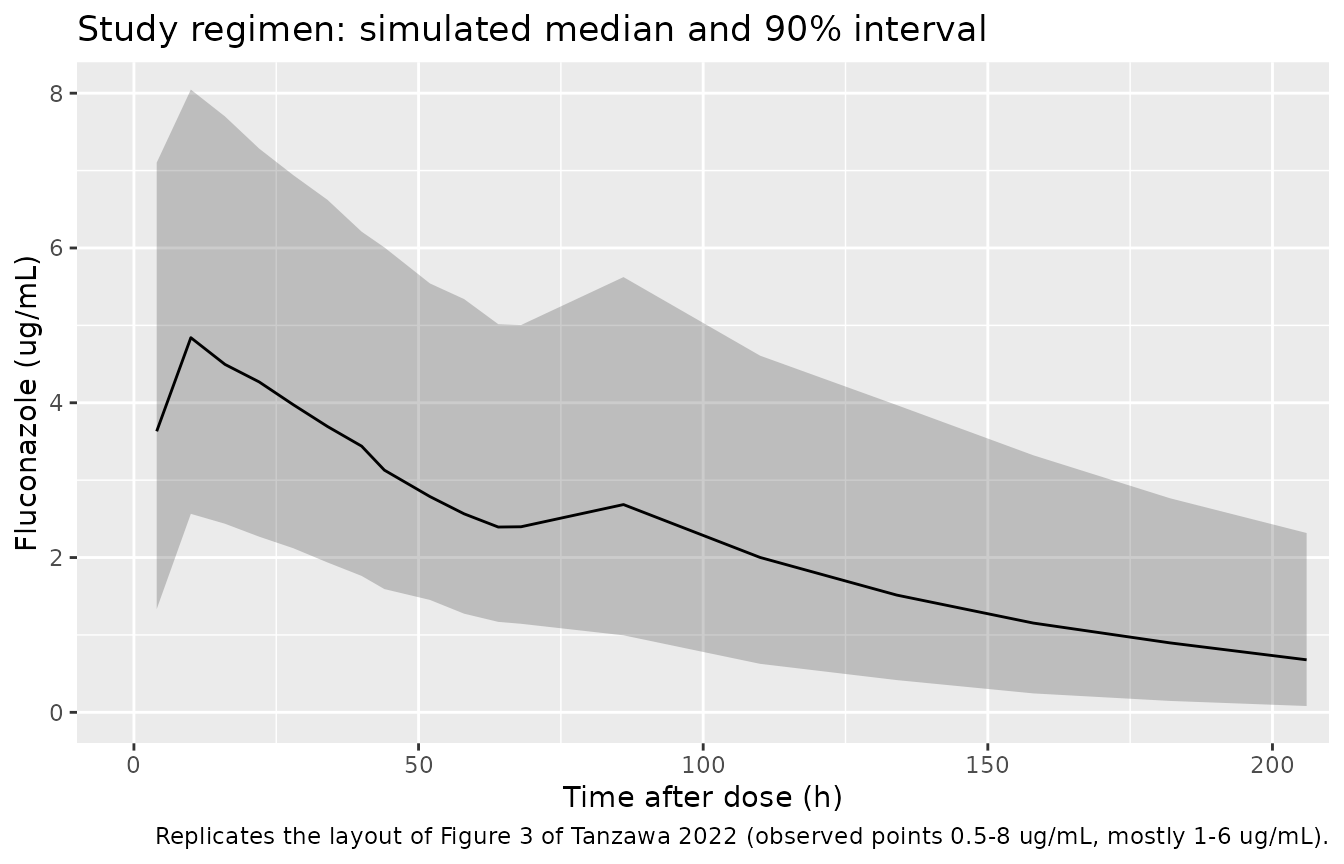
The Results report a median observed concentration of 2.9 ug/mL (IQR 2.2-4.1) in samples taken a median of 42.2 h (IQR 18.5-61.5) after the latest dose. The matching simulated window gives:

during_treatment <- study_sim |>
  dplyr::filter(time > 0, time <= end_of_dosing, tad >= 18.5, tad <= 61.5)
study_q <- stats::quantile(during_treatment$sim, c(0.25, 0.5, 0.75))
knitr::kable(
  tibble::tibble(
    Statistic = c("25th percentile", "Median", "75th percentile"),
    `Simulated (ug/mL)` = round(unname(study_q), 2),
    `Observed (ug/mL)` = c(2.2, 2.9, 4.1)
  )
)

Statistic	Simulated (ug/mL)	Observed (ug/mL)
25th percentile	2.45	2.2
Median	3.35	2.9
75th percentile	4.44	4.1

# Realised median about 3.35 ug/mL (+16%). The reconstructed cohort's PMA
# during dosing (median about 25 weeks) sits below the Table 1 study-period
# median of 28.5 weeks, which lowers CL and raises concentrations. A wrong CL,
# V or dose unit moves this median by far more than 30%.
stopifnot(abs(study_q[["50%"]] / 2.9 - 1) < 0.3)

Assumptions and deviations

Conversion rate constant kc encoded as fixed. Table 3 prints theta_kc = 0.43 /h identically in the base model, the final model and the bootstrap median, with a zero-width bootstrap 95% CI (0.43 to 0.43). The base model column gives it no RSE. The final model column’s “5.40%” RSE copies the V row exactly, as do all of that column’s RSEs, which repeat the base model’s (see the next item). An estimated parameter that the Results describe as poorly informed (“limited number of samples during the conversion phase”) would not bootstrap to a single value, so the maintainers read kc as held constant and wrap it in fixed(). The paper does not say where 0.43 /h came from. Simulations are unaffected either way.
Final model RSE column. Every RSE in the Table 3 final model column (10.59, 5.40, 5.40, 34.8, 49.2, 12.8, 70.7%) repeats the base model column, and the three covariate exponents have none. These look like table-assembly slips. The point estimates match the bootstrap medians and are used as printed.
IIV scale. Table 3 reports IIV only as CV%. It is converted with the log-normal identity omega^2 = log(1 + CV^2) (CL 28.1% gives 0.0760, V 15.8% gives 0.0247). The alternative omega^2 = CV^2 differs by under 2% at these magnitudes.
Residual error. Phoenix NLME’s additive-plus-multiplicative error with a 14.0% proportional CV and a 0.068 ug/mL additive SD is encoded as add(0.068) + prop(0.14), with the variances summing.
Allometry is unnormalized. CL is per kg^0.75 and V per kg, with weight in kg and no reference weight. The PMA, SCr and ALP ratios use the paper’s references of 29 weeks, 0.64 mg/dL and 958 IU/L. PMA is carried in weeks.
ALP units. Table 1 prints “IU/mL”; the values (median 958) and the Discussion’s 100-2,000 IU/L range show this is IU/L.
Table 4 prose vs table. The Results quote q72h trough percentiles of 3.5 (2.1-5.6), 2.7 (1.6-4.1) and 2.1 (1.2-3.2) ug/mL, wider than Table 4’s 3.5 (2.2-4.9), 2.7 (1.7-4.0) and 2.1 (1.3-3.0). The medians agree. The comparison uses the Table 4 medians.
Simulated covariate distributions. The paper does not state the distributions its Monte Carlo used. PMA, weight, SCr and ALP were reconstructed from Table 1 as described under Virtual cohorts. PMA bounds of 23-28, 29-36 and 37-39 weeks stand in for the paper’s open-ended groups. The steady-state comparison is insensitive to the weight assumption; the PTA values depend on the SCr and PMA spreads and are compared on their trend.
Study-regimen cohort. For the VPC the maintainers assumed gestational age interpolated through the Table 1 median and IQR (extremes 22.9-27.9 weeks), birth weight log-normal around 748 g, 15 g/kg/day growth from birth, time-constant SCr and ALP per infant, a 0.5 h infusion, and dosing for the 17-day median treatment duration. The paper does not report actual infusion durations.
Table 4 not reproduced in level. The simulated steady-state medians are about 20% below Table 4, and the Table 4 percentiles and SCr-stratified PTA imply less between-infant variability than the reported IIV. The comparison is shown in full, and the gate uses the level-independent accumulation ratios and the PTA trends. See the steady-state section for the arithmetic.
Covariates screened but not retained (PNA, height and albumin) are listed in the model’s covariatesDataExcluded metadata with their Table 2 OFV changes.
No correction notice for this article was found in Europe PMC as of 2026-10-01. The supplement holds only Figures S1-S2 (CL against SCr, and goodness of fit by postnatal age band) and no parameter values.