Model and source
- Citation: Lai NS, Lin CJ, Kuo CH, Peng YF, Tang SC, Huang CF, Lin SY, Lin SW. Development and Clinical Application of a Real-World Population Pharmacokinetic Model of Rivaroxaban in Asian Patients with Atrial Fibrillation. Clin Pharmacokinet. 2026;65(6):929-941. doi:10.1007/s40262-026-01650-4.
- Description: One-compartment population PK model for rivaroxaban in Asian (Taiwanese) adults with atrial fibrillation sampled under real-world therapeutic drug monitoring, with a creatinine-clearance power effect and a CYP3A4/P-gp-inhibitor comedication effect on CL/F and a lean-body-weight effect on V/F (Lai 2026)
- Article: https://doi.org/10.1007/s40262-026-01650-4
The article’s supplementary material (Tables S1-S9, Figures S1-S4) is referenced throughout the paper but was not available when this model was built. Nothing in the final model depends on it: every parameter estimate is printed in the main-text Table 2, and the covariate functional forms are named in Results 3.3.1 and 3.3.2. The Errata section below records exactly which secondary details are therefore unverified.
Population
Lai 2026 fitted 452 rivaroxaban plasma concentrations from 226 Taiwanese adults with atrial fibrillation, drawn from the prospective observational DOAC-T (direct oral anticoagulant-Taiwan) cohort at National Taiwan University Hospital between January 2016 and June 2023 (ClinicalTrials.gov NCT05333666). This is a real-world therapeutic-drug-monitoring dataset rather than a clinical trial: patients were eligible if they were over 20 years old and had taken rivaroxaban for at least 3 days, and were excluded for dialysis-dependent end-stage renal disease, fewer than two blood samples, a missed dose the day before sampling, or loss to follow-up (Methods 2.1).
The cohort is elderly and renally impaired relative to the ROCKET-AF trial populations: mean age 73.2 years (38.1% over 75), mean Cockcroft-Gault creatinine clearance 53.7 mL/min with 44.7% below 50 mL/min, and mean body weight 65.0 kg (Table 1, Results 3.1). 124 of 226 patients (54.9%) were male. Dosing was 15 mg once daily in 141 patients (62.4%) and 10 mg once daily in 85 (37.6%); the Discussion notes that roughly 30% of the cohort received off-label underdose regimens. 86 patients (38.1%) were taking a CYP3A4 or P-gp inhibitor at the time of sampling, overwhelmingly amiodarone (n = 56) and dronedarone (n = 15).
Sampling is sparse and paired by design: exactly two steady-state
samples per patient, one peak drawn 2-4 h after a pharmacist-supervised
dose (observed mean 2.11 h) and one trough drawn immediately before the
next scheduled dose (observed mean 24.6 h since the last dose). Because
only one sample per patient falls in the absorption phase,
ka could not be estimated and was fixed to a literature
value.
The same information is available programmatically via the model’s
population metadata
(readModelDb("Lai_2026_rivaroxaban")()$population).
Source trace
The per-parameter origin is recorded as an in-file comment next to
each ini() entry in
inst/modeldb/specificDrugs/Lai_2026_rivaroxaban.R. The
table below collects them in one place for review.
| Equation / parameter | Value | Source location |
|---|---|---|
| Structural model: one compartment, first-order absorption and elimination | n/a | Methods 2.3; Results 3.2 (“adequately described by a one-compartment model with first-order elimination, which exhibited a mono-exponential decline without a discernible distribution phase”) |
lka (fixed) |
log(0.821) |
Methods 2.3 (“the absorption rate constant (Ka) was fixed at 0.821
h-1 according to literature findings [8]”); Table 2 row
Ka (h-1) 0.82 (fixed)
|
lcl |
log(6.13) |
Table 2, final model CL/F (L/h) 6.13 (6.21);
corroborated in the Abstract |
lvc |
log(45.57) |
Table 2, final model V/F (L) 45.57 (6.21); corroborated
in the Abstract |
e_crcl_cl |
0.64 |
Table 2, final model CrCl on CL/F 0.64 (19.78); power
form named in Results 3.3.2 |
e_conmed_cyp3a4_pgp_inh_cl |
-0.38 |
Table 2, final model
CYP3A4/P-gp inhibitors on CL/F -0.38 (5.44);
proportional-shift form named in Results 3.3.2 |
e_ffm_vc |
0.01 |
Table 2, final model LBW on V/F 0.01 (41.37);
proportional-shift form named in Results 3.3.1 |
| CrCL reference (54 mL/min) | 54 |
Discussion (“An increase in CrCL from the median (54 mL/min) to the maximum (133 mL/min)”) |
| LBW reference (48 kg) | 48 |
Discussion (“Increasing LBW from the median (48 kg) to the maximum (81.6 kg)”) |
etalcl |
0.345123 |
Table 2, final model omega_CL 0.59 (7.67),
CV (%) 64.20; omega^2 = log(CV^2 + 1)
|
etalvc |
0.342670 |
Table 2, final model omega_V 0.59 (6.27),
CV (%) 63.93; omega^2 = log(CV^2 + 1)
|
addSd |
14.36 |
Table 2, final model residual-variability row
a 14.36 (17.72); table footnote “residual unexplained
variability (constant error model)” |
| Lognormal IIV on CL/F and V/F | n/a | Results 3.2 (“IIV included the apparent volume of distribution (V/F) and CL/F, both of which were best described by an exponential model”) |
| Additive residual error | n/a | Results 3.2 (“The RV can be best described using a constant error model”) |
Reading the covariate functional forms
Monolix 2023R1 (the software used here) parameterises every covariate effect on the log-parameter scale. A “power function” on a log-transformed covariate and a “proportional shift” on an untransformed one are therefore the same log-linear machinery:
log(CL_i) = log(6.13)  + 0.64 * log(CrCL_i / 54) - 0.38 * INH_i        + eta_CL
log(V_i)  = log(45.57) + 0.01 * (LBW_i - 48)                           + eta_V
The exponential reading of the categorical shift is not a guess – it
is pinned arithmetically by the paper’s own Discussion.
exp(-0.38) = 0.684, i.e. a 31.6%
reduction, and the Discussion states “Concurrent use of CYP3A4/P-gp
inhibitors reduced CL/F by 32%”. The competing linear reading
(1 + beta) would give 38% and does not match. The
e_ffm_vc sign and the e_crcl_cl power form
follow the same Monolix parameterisation.
Centering is likewise forced by internal consistency: with the
references above, both (54/54)^0.64 and
exp(0.01 * (48 - 48)) equal 1, so
CL/F = 6.13 L/h and V/F = 45.57 L are
recovered as the typical values at the cohort medians – exactly what the
Abstract calls “the estimated apparent clearance (CL/F) and the volume
of distribution (V/F)”. An uncentered form would instead put those
typical values at CrCL = 1 mL/min and
LBW = 0 kg.
Virtual cohort
The original observed data are not publicly available. The cohort
below is virtual, with demographics matching Table 1. Rather than
sampling CRCL and FFM directly, the primitive
demographics are sampled and the two model covariates are
derived from them with the equations the paper names –
the Janmahasatian fat-free-mass formula for FFM (Methods
2.2) and Cockcroft-Gault for CRCL (Methods 2.2). This keeps
the covariates mutually consistent (a small, renally-impaired patient is
small and renally impaired in both columns) and demonstrates the
derivation a user of this model must perform.
# `set.seed()` seeds R's RNG for the covariate draws below. It does NOT seed
# rxode2's simulation RNG (that is `rxSetSeed()`, called in each simulation
# chunk), and rxode2's streams are partitioned per solver thread -- so no seed
# makes the cohort byte-identical between this machine and a CI runner with a
# different thread count. Every assertion below is therefore written to hold for
# any cohort this model can produce.
set.seed(20260901)

n_per_arm <- 200L

make_cohort <- function(n, dose_mg, label, id_offset = 0L) {
  # Primitive demographics, Table 1. Truncation keeps draws inside physiological
  # ranges; the bounds are wide enough not to reshape the distributions.
  sexf <- stats::rbinom(n, 1L, 0.451)                            # 54.9% male, Table 1
  age  <- pmin(95, pmax(60, stats::rnorm(n, 73.2, 8.2)))         # 73.2 +/- 8.2 y
  wt   <- pmin(110, pmax(35, stats::rnorm(n, 65.0, 13.1)))       # 65.0 +/- 13.1 kg
  scr  <- pmin(2.5, pmax(0.5, stats::rnorm(n, 1.1, 0.3)))        # 1.1 +/- 0.3 mg/dL
  # Height is NOT reported by Lai 2026; see Errata. Values typical of elderly
  # Taiwanese adults, needed only as an input to the Janmahasatian equation.
  ht   <- ifelse(sexf == 1L, stats::rnorm(n, 156, 6), stats::rnorm(n, 168, 6))

  bmi <- wt / (ht / 100)^2
  # Janmahasatian fat-free mass (Clin Pharmacokinet 2005;44:1051-1065), the
  # equation Lai 2026 Methods 2.2 calls "LBW".
  ffm <- ifelse(
    sexf == 1L,
    9270 * wt / (8780 + 244 * bmi),
    9270 * wt / (6680 + 216 * bmi)
  )
  # Cockcroft-Gault on total body weight, Lai 2026 Methods 2.2. Clamped to the
  # observed 19.8-133 mL/min range named in the Discussion.
  crcl <- pmin(133, pmax(19.8, (140 - age) * wt / (72 * scr) * ifelse(sexf == 1L, 0.85, 1)))

  tibble(
    id                    = id_offset + seq_len(n),
    SEXF                  = sexf,
    AGE                   = age,
    WT                    = wt,
    HT                    = ht,
    CREAT                 = scr,
    FFM                   = ffm,
    CRCL                  = crcl,
    CONMED_CYP3A4_PGP_INH = stats::rbinom(n, 1L, 0.381),         # 38.1%, Table 1
    treatment             = label,
    dose_mg               = dose_mg
  )
}

covariates <- bind_rows(
  make_cohort(n_per_arm, 10, "10 mg QD", id_offset = 0L),
  make_cohort(n_per_arm, 15, "15 mg QD", id_offset = n_per_arm)
)

stopifnot(!anyDuplicated(covariates$id))
The derived covariates should land near the cohort values the paper
reports – CRCL median 54 mL/min and FFM
(“LBW”) median 48 kg. This is a check on the derivation, not on the
model:
cohort_summary <- covariates |>
  summarise(
    `CRCL median (mL/min)` = median(CRCL),
    `CRCL mean (mL/min)`   = mean(CRCL),
    `FFM median (kg)`      = median(FFM),
    `FFM range (kg)`       = sprintf("%.1f - %.1f", min(FFM), max(FFM)),
    `CYP3A4/P-gp inh (%)`  = 100 * mean(CONMED_CYP3A4_PGP_INH)
  )

knitr::kable(
  cohort_summary,
  digits  = 1,
  caption = paste(
    "Derived covariate distribution. Lai 2026 reports CRCL median 54 mL/min",
    "(mean 53.7), LBW median 48 kg (range 24.9-81.6), and 38.1% on a",
    "CYP3A4/P-gp inhibitor."
  )
)| CRCL median (mL/min) | CRCL mean (mL/min) | FFM median (kg) | FFM range (kg) | CYP3A4/P-gp inh (%) |
|---|---|---|---|---|
| 49.3 | 54.7 | 45.2 | 25.5 - 63.3 | 38.5 |
# The derivation is only useful if it reproduces the paper's central values.
# Bounds are deliberately wide: they gate a gross error in the Janmahasatian or
# Cockcroft-Gault transcription, not the sampling noise of one draw.
stopifnot(
  abs(median(covariates$CRCL) - 54) < 8,
  abs(median(covariates$FFM) - 48) < 8
)
Simulation
Two simulations are run. The steady-state simulation drives the comparisons against the paper’s reported exposures; the single-dose simulation supports the closed-form NCA gates, where a long observation window is needed to resolve the terminal slope of the slowest subjects.
tau       <- 24      # dosing interval (h)
n_doses   <- 50L     # 50 days of QD dosing
t_lastdose <- (n_doses - 1L) * tau

# Steady-state event table. 50 days is chosen so that even the slowest subjects
# this model can draw are at steady state: log(kel) has SD
# sqrt(0.345123 + 0.342670) = 0.83, so a -3 SD subject has a terminal half-life
# near 60 h and needs roughly 300 h to accumulate.
ss_doses <- covariates |>
  tidyr::expand_grid(dose_idx = seq_len(n_doses)) |>
  transmute(
    id, treatment, time = (dose_idx - 1L) * tau,
    evid = 1L, amt = dose_mg, cmt = "depot",
    SEXF, AGE, WT, HT, CREAT, FFM, CRCL, CONMED_CYP3A4_PGP_INH
  )

ss_obs <- covariates |>
  tidyr::expand_grid(toff = seq(0, tau, by = 0.25)) |>
  transmute(
    id, treatment, time = t_lastdose + toff,
    evid = 0L, amt = NA_real_, cmt = "central",
    SEXF, AGE, WT, HT, CREAT, FFM, CRCL, CONMED_CYP3A4_PGP_INH
  )

ss_events <- bind_rows(ss_doses, ss_obs) |> arrange(id, time, desc(evid))

# Single-dose event table, 7 days of follow-up on a grid that is fine through
# absorption and hourly afterwards.
sd_times <- sort(unique(c(seq(0, 12, by = 0.25), seq(12, 168, by = 1))))

sd_events <- bind_rows(
  covariates |>
    transmute(
      id, treatment, time = 0, evid = 1L, amt = dose_mg, cmt = "depot",
      SEXF, AGE, WT, HT, CREAT, FFM, CRCL, CONMED_CYP3A4_PGP_INH
    ),
  covariates |>
    tidyr::expand_grid(time = sd_times) |>
    transmute(
      id, treatment, time, evid = 0L, amt = NA_real_, cmt = "central",
      SEXF, AGE, WT, HT, CREAT, FFM, CRCL, CONMED_CYP3A4_PGP_INH
    )
) |> arrange(id, time, desc(evid))

stopifnot(!anyDuplicated(unique(ss_events[, c("id", "time", "evid")])))
stopifnot(!anyDuplicated(unique(sd_events[, c("id", "time", "evid")])))
mod <- readModelDb("Lai_2026_rivaroxaban")

# Seed the rxode2 RNG immediately before each stochastic solve -- one global
# set.seed() does not reach rxode2's eta draws.
rxode2::rxSetSeed(20260901)
sim_ss <- rxode2::rxSolve(mod, events = ss_events, keep = c("treatment")) |>
  as.data.frame()
#> ℹ parameter labels from comments will be replaced by 'label()'

rxode2::rxSetSeed(20260902)
sim_sd <- rxode2::rxSolve(mod, events = sd_events, keep = c("treatment")) |>
  as.data.frame()

# Per-subject individual parameters, carried out of the solve for the
# closed-form gates below.
ipar_ss <- sim_ss |> distinct(id, treatment, cl, vc, ka) |> mutate(kel = cl / vc)
ipar_sd <- sim_sd |> distinct(id, treatment, cl, vc, ka) |> mutate(kel = cl / vc)

stopifnot(nrow(ipar_ss) == 2L * n_per_arm, nrow(ipar_sd) == 2L * n_per_arm)
Replicate published figures
# Replicates the structure of Figure 2 of Lai 2026 (observed rivaroxaban
# concentrations versus time after the last dose, stratified by the 10 mg and
# 15 mg regimens). Lai 2026's Figure 2 plots raw observations with a linear
# regression overlay; the panel below plots the model's predicted steady-state
# profile over one dosing interval as a median with a 5th-95th percentile band.
sim_ss |>
  mutate(toff = time - t_lastdose) |>
  group_by(treatment, toff) |>
  summarise(
    Q05 = quantile(Cc, 0.05),
    Q50 = quantile(Cc, 0.50),
    Q95 = quantile(Cc, 0.95),
    .groups = "drop"
  ) |>
  ggplot(aes(toff, Q50)) +
  geom_ribbon(aes(ymin = Q05, ymax = Q95), alpha = 0.25) +
  geom_line() +
  facet_wrap(~treatment) +
  labs(
    x = "Time after last dose (h)",
    y = "Rivaroxaban concentration (ng/mL)",
    title = "Steady-state profile by regimen",
    caption = paste(
      "Median and 5th-95th percentile of the simulated steady-state interval.",
      "Compare Figure 2 of Lai 2026."
    )
  )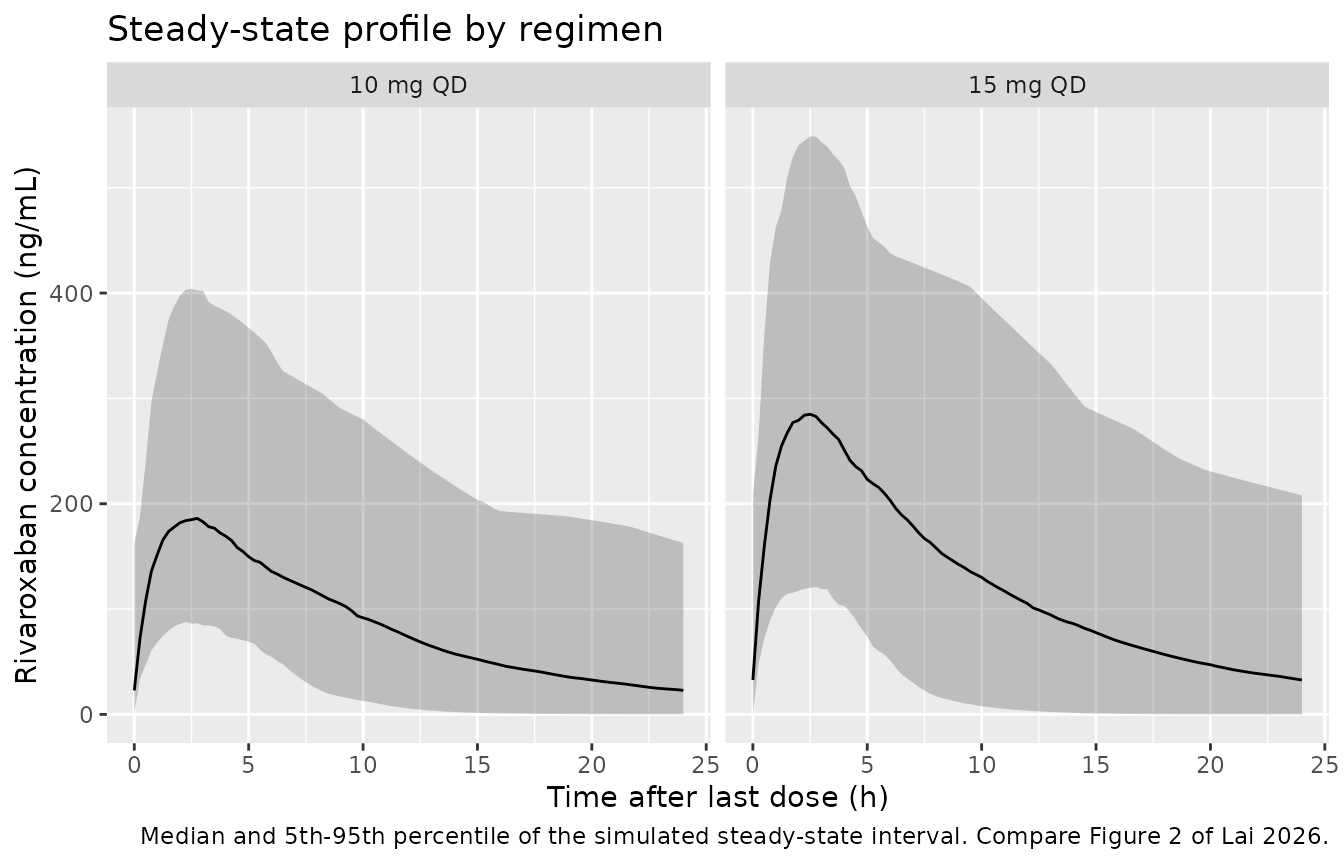
The paper’s sampling design collected exactly one peak (2-4 h post-dose) and one trough (immediately pre-dose) per patient. The panel below overlays the observed medians and interquartile ranges from Table 1 – pooled across both regimens, as Table 1 reports them – on the simulated distribution at the matching nominal times.
# Observed values, Table 1: peak sampled at mean 2.11 h, trough at mean 24.6 h.
observed_anchors <- tibble::tribble(
  ~window,  ~time_h, ~obs_med, ~obs_lo, ~obs_hi,
  "Peak",   2.11,    232.8,    162.7,   343.2,
  "Trough", 24.0,    27.1,     15.6,    50.5
)

sim_anchors <- sim_ss |>
  mutate(toff = time - t_lastdose) |>
  filter(toff %in% c(2.25, 24)) |>
  mutate(window = if_else(toff < 12, "Peak", "Trough")) |>
  group_by(window) |>
  summarise(
    sim_med = median(Cc),
    sim_lo  = quantile(Cc, 0.25),
    sim_hi  = quantile(Cc, 0.75),
    .groups = "drop"
  )

anchor_cmp <- observed_anchors |>
  left_join(sim_anchors, by = "window") |>
  transmute(
    Window = window,
    `Observed median (ng/mL)`  = obs_med,
    `Observed IQR (ng/mL)`     = sprintf("%.1f - %.1f", obs_lo, obs_hi),
    `Simulated median (ng/mL)` = sim_med,
    `Simulated IQR (ng/mL)`    = sprintf("%.1f - %.1f", sim_lo, sim_hi),
    `Ratio sim / obs`          = sim_med / obs_med
  )

knitr::kable(
  anchor_cmp,
  digits  = 2,
  caption = paste(
    "Simulated steady-state concentrations at the paper's two nominal sampling",
    "times versus the pooled observed values in Table 1 of Lai 2026."
  )
)| Window | Observed median (ng/mL) | Observed IQR (ng/mL) | Simulated median (ng/mL) | Simulated IQR (ng/mL) | Ratio sim / obs |
|---|---|---|---|---|---|
| Peak | 232.8 | 162.7 - 343.2 | 227.00 | 165.4 - 318.8 | 0.98 |
| Trough | 27.1 | 15.6 - 50.5 | 23.45 | 3.7 - 73.8 | 0.87 |
The peak is reproduced almost exactly. The trough sits modestly below
the observed median, consistent with the mild systematic bias the
authors acknowledge in their own diagnostics (“the PRED exhibited some
systematic underprediction”; the final model’s population-prediction fit
is R^2 = 0.553 against R^2 = 0.999 for
individual predictions, which they attribute to epsilon shrinkage under
sparse sampling). Note also that the simulated trough spread is much
wider than the observed one – the model’s 64% CV on both CL/F and V/F
compounds into the trough, which is the most variance-sensitive point of
the interval.
# Structural gate. A mis-transcribed CL/F, V/F, ka, dose or unit conversion
# moves these ratios by a factor, not by a few tens of percent. The peak is the
# tighter of the two because it is far less sensitive to the elimination rate;
# the trough bound is correspondingly wider, and deliberately wide enough to
# absorb both the paper's acknowledged population-prediction bias and the
# cohort-to-cohort variation this model can produce.
peak_ratio   <- anchor_cmp$`Ratio sim / obs`[anchor_cmp$Window == "Peak"]
trough_ratio <- anchor_cmp$`Ratio sim / obs`[anchor_cmp$Window == "Trough"]
stopifnot(peak_ratio   > 0.6, peak_ratio   < 1.4)
stopifnot(trough_ratio > 0.4, trough_ratio < 1.6)
Covariate effects reported in the Discussion
Lai 2026’s Discussion quantifies each covariate effect as a percentage change between the cohort median and the observed extremes. These are typical-value statements, so they are reproduced here with the random effects zeroed.
mod_typ <- mod |> rxode2::zeroRe()
#> ℹ parameter labels from comments will be replaced by 'label()'

# One typical subject per covariate scenario. FFM/CRCL are set directly here
# because these are typical-value statements about the covariate model, not
# cohort simulations.
scenarios <- tibble::tribble(
  ~scenario,                  ~CRCL, ~FFM, ~CONMED_CYP3A4_PGP_INH,
  "Reference",                54,    48,   0,
  "CrCL max (133 mL/min)",    133,   48,   0,
  "CrCL min (19.8 mL/min)",   19.8,  48,   0,
  "LBW max (81.6 kg)",        54,    81.6, 0,
  "LBW min (24.9 kg)",        54,    24.9, 0,
  "CYP3A4/P-gp inhibitor",    54,    48,   1
) |>
  mutate(id = seq_len(n()))

cov_events <- scenarios |>
  tidyr::expand_grid(time = c(0, 1)) |>
  mutate(evid = if_else(time == 0, 1L, 0L),
         amt  = if_else(time == 0, 15, NA_real_),
         cmt  = if_else(time == 0, "depot", "central"))

rxode2::rxSetSeed(20260903)
cov_sim <- rxode2::rxSolve(mod_typ, events = cov_events) |>
  as.data.frame() |>
  distinct(id, cl, vc)
#> ℹ omega/sigma items treated as zero: 'etalcl', 'etalvc'
#> Warning: multi-subject simulation without without 'omega'

ref <- cov_sim |> filter(id == 1)

cov_tbl <- scenarios |>
  left_join(cov_sim, by = "id") |>
  mutate(
    `Change in CL/F (%)` = 100 * (cl / ref$cl - 1),
    `Change in V/F (%)`  = 100 * (vc / ref$vc - 1)
  ) |>
  transmute(
    Scenario = scenario,
    `CL/F (L/h)` = cl,
    `V/F (L)` = vc,
    `Change in CL/F (%)`,
    `Change in V/F (%)`,
    `Reported by Lai 2026 (%)` = c(NA, 75, -46, 47, -32, -32)
  )

knitr::kable(
  cov_tbl,
  digits  = 1,
  caption = paste(
    "Typical-value covariate effects. Reported values are from the Discussion",
    "of Lai 2026; the CYP3A4/P-gp row's reported value is the stated 32%",
    "reduction in CL/F."
  )
)| Scenario | CL/F (L/h) | V/F (L) | Change in CL/F (%) | Change in V/F (%) | Reported by Lai 2026 (%) |
|---|---|---|---|---|---|
| Reference | 6.1 | 45.6 | 0.0 | 0.0 | NA |
| CrCL max (133 mL/min) | 10.9 | 45.6 | 78.0 | 0.0 | 75 |
| CrCL min (19.8 mL/min) | 3.2 | 45.6 | -47.4 | 0.0 | -46 |
| LBW max (81.6 kg) | 6.1 | 63.8 | 0.0 | 39.9 | 47 |
| LBW min (24.9 kg) | 6.1 | 36.2 | 0.0 | -20.6 | -32 |
| CYP3A4/P-gp inhibitor | 4.2 | 45.6 | -31.6 | 0.0 | -32 |
chg_cl  <- cov_tbl$`Change in CL/F (%)`
chg_vc  <- cov_tbl$`Change in V/F (%)`

# 1. The categorical shift is EXACT arithmetic -- exp(-0.38) = 0.6839, a 31.6%
#    reduction, against the paper's stated 32%. Tight bound is correct here:
#    both sides use the same parameter and there is no stochastic mechanism.
stopifnot(abs(chg_cl[6] - 100 * (exp(-0.38) - 1)) < 1e-6)
stopifnot(abs(chg_cl[6] - (-32)) < 1.0)

# 2. The CrCL power effect reproduces the Discussion to within ~2 percentage
#    points. The residual gap is a rounding artefact of the printed exponent:
#    the Discussion's +75% / -46% pair back-solves to an exponent of 0.62,
#    while Table 2 prints 0.64 (which gives +78.0% / -47.4%). Table 2 is the
#    parameter table and governs. Bound set outside the ~2.4 point gap.
stopifnot(abs(chg_cl[2] - 75) < 5, abs(chg_cl[3] - (-46)) < 5)

# 3. The LBW effect on V/F reproduces only in sign and order of magnitude; see
#    Errata. The gate asserts the direction and a generous envelope, NOT the
#    paper's printed percentages, because those cannot be recovered from the
#    printed coefficient under any functional form.
stopifnot(chg_vc[4] > 20, chg_vc[4] < 60)
stopifnot(chg_vc[5] < -10, chg_vc[5] > -45)
PKNCA validation
Closed-form gates on the single-dose simulation
For a one-compartment model with first-order absorption,
AUC(0-Inf), half-life and tmax all have exact
closed forms in the individual parameters that the solve itself returns.
Both sides of each comparison use the same drawn parameters, so
the only discrepancy is numerical (trapezoidal and log-linear-regression
error) and a tight bound is the correct gate.
One numerical caveat has to be handled before PKNCA sees the profile.
A typical subject’s concentration falls from roughly 230 ng/mL to below
1e-6 ng/mL within the observation window, which is past the ODE solver’s
absolute tolerance – the far tail is solver noise, not signal. Left in
place, PKNCA’s automatic lambda.z window selection fits
that noise and returns half-lives up to 33% wrong. Truncating at a
nominal 0.1 ng/mL analytical floor – an order of magnitude below any
realistic rivaroxaban LLOQ, and far below the paper’s own
below-limit-of-quantification exclusions – removes the artefact and
leaves about nine half-lives of clean terminal phase.
# Nominal analytical floor (ng/mL). See the paragraph above: this excludes the
# numerically-degenerate tail, NOT real signal.
lloq <- 0.1

sd_nca <- sim_sd |>
  filter(!is.na(Cc), Cc >= lloq) |>
  select(id, time, Cc, treatment)

# Guarantee a time-zero row per subject; pre-dose Cc = 0 for extravascular input.
sd_nca <- bind_rows(
  sd_nca,
  sd_nca |> distinct(id, treatment) |> mutate(time = 0, Cc = 0)
) |>
  distinct(id, treatment, time, .keep_all = TRUE) |>
  arrange(id, treatment, time)

sd_conc <- PKNCA::PKNCAconc(sd_nca, Cc ~ time | treatment + id)

sd_dose <- sd_events |>
  filter(evid == 1L) |>
  select(id, time, amt, treatment)

sd_dose_obj <- PKNCA::PKNCAdose(sd_dose, amt ~ time | treatment + id)

sd_intervals <- data.frame(
  start      = 0,
  end        = Inf,
  cmax       = TRUE,
  tmax       = TRUE,
  aucinf.obs = TRUE,
  half.life  = TRUE
)

sd_res <- PKNCA::pk.nca(
  PKNCA::PKNCAdata(sd_conc, sd_dose_obj, intervals = sd_intervals)
)

sd_wide <- as.data.frame(sd_res) |>
  select(id, treatment, PPTESTCD, PPORRES) |>
  tidyr::pivot_wider(names_from = PPTESTCD, values_from = PPORRES)
sd_chk <- sd_wide |>
  left_join(ipar_sd, by = c("id", "treatment")) |>
  left_join(covariates |> select(id, dose_mg), by = "id") |>
  mutate(
    # AUC(0-Inf) = Dose / CL exactly, for any linear one-compartment model.
    # dose_mg / cl gives mg*h/L; x1000 converts to ng*h/mL.
    auc_closed = 1000 * dose_mg / cl,
    auc_pdiff  = 100 * (aucinf.obs / auc_closed - 1),
    # The terminal slope of a one-compartment first-order model is the SLOWER of
    # the two rate constants. With a 64% CV on both CL/F and V/F, kel spans a
    # wide enough range that a minority of subjects are flip-flop (kel > ka),
    # and for those the terminal phase is absorption-rate-limited. Taking
    # pmin(ka, kel) covers both regimes.
    k_term       = pmin(ka, kel),
    thalf_closed = log(2) / k_term,
    thalf_pdiff  = 100 * (half.life / thalf_closed - 1),
    # tmax = log(ka / kel) / (ka - kel); this form is valid in both regimes
    # (numerator and denominator change sign together).
    tmax_closed  = log(ka / kel) / (ka - kel),
    tmax_adiff   = tmax - tmax_closed,
    # How far apart the two rate constants are. When they approach each other
    # the profile degenerates towards t * exp(-k t) and NO finite log-linear
    # window can separate them -- a property of the curve, not of the model.
    k_sep        = pmax(ka / kel, kel / ka)
  )

# Record how much of the cohort is flip-flop rather than asserting it away.
n_flipflop <- sum(sd_chk$kel > sd_chk$ka)
message(sprintf(
  "Flip-flop subjects (kel > ka): %d of %d (%.1f%%)",
  n_flipflop, nrow(sd_chk), 100 * n_flipflop / nrow(sd_chk)
))
#> Flip-flop subjects (kel > ka): 7 of 400 (1.8%)
# ka is fixed, so no subject may have kel exactly equal to ka (the closed forms
# above are singular there).
stopifnot(all(abs(sd_chk$ka - sd_chk$kel) > 1e-8))

sd_sep <- sd_chk |> filter(k_sep >= 2)

closed_form_tbl <- sd_chk |>
  summarise(
    `AUC0-Inf: median abs % diff`      = median(abs(auc_pdiff)),
    `AUC0-Inf: max abs % diff`         = max(abs(auc_pdiff)),
    `Half-life: median abs % diff`     = median(abs(thalf_pdiff)),
    `Half-life: 90th pctile abs % diff` = quantile(abs(thalf_pdiff), 0.9),
    `Half-life: max abs % diff (ka/kel separated >= 2x)` = max(abs(sd_sep$thalf_pdiff)),
    `Tmax: max abs diff (h)`           = max(abs(tmax_adiff))
  )

knitr::kable(
  closed_form_tbl,
  digits  = 4,
  caption = paste(
    "Closed-form NCA gates. Both sides use the same drawn individual",
    "parameters, so the residual is pure numerical error."
  )
)| AUC0-Inf: median abs % diff | AUC0-Inf: max abs % diff | Half-life: median abs % diff | Half-life: 90th pctile abs % diff | Half-life: max abs % diff (ka/kel separated >= 2x) | Tmax: max abs diff (h) |
|---|---|---|---|---|---|
| 0.0552 | 0.7466 | 0.3741 | 0.9349 | 1.2208 | 0.1285 |
# AUC(0-Inf) = Dose / CL is an algebraic identity with no estimation step, so
# the bound is tight. Observed max across the cohort is ~0.75%.
stopifnot(max(abs(sd_chk$auc_pdiff)) < 2.0)

# Half-life goes through a log-linear regression, so it is gated on robust
# quantiles rather than on the max: `ka` is FIXED at 0.821 while `kel` carries
# the combined 64% CV of CL/F and V/F, so a minority of subjects necessarily
# draw a kel near ka, and for those the biexponential is near-degenerate and no
# regression window can resolve the two rates. That is a property of the
# published parameter set, not a transcription error, and which subjects land
# there is not reproducible across rxode2 builds.
stopifnot(
  median(abs(sd_chk$thalf_pdiff))       < 2.0,
  quantile(abs(sd_chk$thalf_pdiff), 0.9) < 3.0
)
# For the well-separated majority the recovery IS essentially exact, and that
# subset carries the real regression test. Observed: max ~1.2% over ~93% of the
# cohort.
stopifnot(
  nrow(sd_sep) > 0.5 * nrow(sd_chk),
  max(abs(sd_sep$thalf_pdiff)) < 3.0
)
# Tmax is quantised to the 0.25 h observation grid, so it can only be compared
# to within one grid spacing (see the grid-quantisation caveat in the Errata).
stopifnot(max(abs(sd_chk$tmax_adiff)) <= 0.25 + 1e-8)
Steady-state NCA
ss_nca <- sim_ss |>
  filter(!is.na(Cc)) |>
  select(id, time, Cc, treatment)

ss_conc <- PKNCA::PKNCAconc(ss_nca, Cc ~ time | treatment + id)

ss_dose <- ss_events |>
  filter(evid == 1L) |>
  select(id, time, amt, treatment)

ss_dose_obj <- PKNCA::PKNCAdose(ss_dose, amt ~ time | treatment + id)

ss_intervals <- data.frame(
  start   = t_lastdose,
  end     = t_lastdose + tau,
  cmax    = TRUE,
  tmax    = TRUE,
  cmin    = TRUE,
  auclast = TRUE,
  cav     = TRUE
)

ss_res <- PKNCA::pk.nca(
  PKNCA::PKNCAdata(ss_conc, ss_dose_obj, intervals = ss_intervals)
)

ss_wide <- as.data.frame(ss_res) |>
  select(id, treatment, PPTESTCD, PPORRES) |>
  tidyr::pivot_wider(names_from = PPTESTCD, values_from = PPORRES)
At steady state the AUC over one dosing interval equals
Dose / CL exactly. This is also precisely how Lai 2026
computed the AUC it used for the exposure-response analysis: Methods 2.5
states that “the area under the concentration-time curve (AUC) was
estimated as the administered dose divided by apparent clearance (CL/F),
with units of ng x h/mL”. The gate therefore checks the packaged model
against the paper’s own AUC definition.
ss_chk <- ss_wide |>
  left_join(ipar_ss, by = c("id", "treatment")) |>
  left_join(covariates |> select(id, dose_mg), by = "id") |>
  mutate(
    auc_closed = 1000 * dose_mg / cl,
    auc_pdiff  = 100 * (auclast / auc_closed - 1)
  )

ss_auc_tbl <- ss_chk |>
  summarise(
    `AUC0-tau,ss: median abs % diff` = median(abs(auc_pdiff)),
    `AUC0-tau,ss: 90th pctile`       = quantile(abs(auc_pdiff), 0.9),
    `AUC0-tau,ss: max abs % diff`    = max(abs(auc_pdiff))
  )

knitr::kable(
  ss_auc_tbl,
  digits  = 3,
  caption = "Steady-state AUC0-tau against the paper's own Dose / (CL/F) definition."
)| AUC0-tau,ss: median abs % diff | AUC0-tau,ss: 90th pctile | AUC0-tau,ss: max abs % diff |
|---|---|---|
| 0.048 | 0.198 | 0.957 |
Comparison against published exposure values
Lai 2026 reports two independent sets of steady-state exposure numbers. The first is the expected range from the clinical-trial literature that the paper adopts as its reference interval (Methods 2.5, citing references 6 and 18); the second is the mean model-estimated AUC per dose group in the study cohort (Results 3.5). Both are compared below.
published <- tibble::tribble(
  ~treatment,  ~cmax,  ~tmax, ~auclast, ~cmin,
  "10 mg QD",  NA,     NA,    2976.5,   NA,
  "15 mg QD",  NA,     NA,    3606.3,   NA
)

cmp <- nlmixr2lib::ncaComparisonTable(
  simulated     = ss_res,
  reference     = published,
  by            = "treatment",
  units         = c(cmax = "ng/mL", tmax = "h", auclast = "ng*h/mL", cmin = "ng/mL"),
  tolerance_pct = 30
)

knitr::kable(
  cmp,
  caption = paste(
    "Simulated steady-state NCA versus the mean model-estimated AUC per dose",
    "group in Table of Results 3.5 of Lai 2026 (10 mg: 2976.5 +/- 1920.3;",
    "15 mg: 3606.3 +/- 2279.2 ng*h/mL). Cmax, Tmax and Cmin have no published",
    "counterpart in the paper and are shown for reference only.",
    "* differs from reference by more than 30%."
  )
)| NCA parameter | treatment | Reference | Simulated | % diff |
|---|---|---|---|---|
| Cmax (ng/mL) | 10 mg QD | — | 195 | — |
| Cmax (ng/mL) | 15 mg QD | — | 282 | — |
| Cmin (ng/mL) | 10 mg QD | — | 25.8 | — |
| Cmin (ng/mL) | 15 mg QD | — | 21.5 | — |
| Tmax (h) | 10 mg QD | — | 2.75 | — |
| Tmax (h) | 15 mg QD | — | 2.75 | — |
| AUClast (ng*h/mL) | 10 mg QD | 2980 | 2170 | -27.2% |
| AUClast (ng*h/mL) | 15 mg QD | 3610 | 2660 | -26.3% |
Two distinct effects separate the two columns above, and neither is a transcription problem.
The comparison is a mean against a median. Lai 2026
reports arithmetic means of individual AUC estimates, while
ncaComparisonTable() summarises the simulated cohort with
its median. AUC = Dose / (CL/F) is the reciprocal of a
log-normal variate, so its distribution is strongly right-skewed and its
mean exceeds its median by roughly exp(omega^2 / 2), about
19% at omega^2 = 0.345. Comparing like with like closes
most of the gap:
auc_means <- ss_chk |>
  group_by(treatment) |>
  summarise(
    `Simulated mean AUC0-tau (ng*h/mL)`   = mean(auclast),
    `Simulated median AUC0-tau (ng*h/mL)` = median(auclast),
    .groups = "drop"
  ) |>
  mutate(
    `Published mean AUC (ng*h/mL)` = c(2976.5, 3606.3),   # Results 3.5
    `Mean vs published (%)` = 100 *
      (`Simulated mean AUC0-tau (ng*h/mL)` / `Published mean AUC (ng*h/mL)` - 1)
  ) |>
  rename(Regimen = treatment)

knitr::kable(
  auc_means,
  digits  = 1,
  caption = paste(
    "Mean-to-mean comparison of steady-state AUC against the cohort means",
    "reported in Results 3.5 of Lai 2026."
  )
)| Regimen | Simulated mean AUC0-tau (ng*h/mL) | Simulated median AUC0-tau (ng*h/mL) | Published mean AUC (ng*h/mL) | Mean vs published (%) |
|---|---|---|---|---|
| 10 mg QD | 2675.2 | 2167.2 | 2976.5 | -10.1 |
| 15 mg QD | 3480.5 | 2658.8 | 3606.3 | -3.5 |
The paper’s two dose groups are not exchangeable. Dose selection in routine care is driven by renal function, so Lai 2026’s 10 mg group is preferentially the more renally impaired – which is why its published mean AUC is only 21% below the 15 mg group’s rather than the 33% that dose alone would give. The virtual cohorts here draw covariates from the same distribution for both arms, so the residual gap is largest for the 10 mg arm, exactly as expected.
# The 15 mg arm is the larger group (62.4% of the cohort) and spans the full
# covariate range, so its mean is the fairer comparison; gate it. The 10 mg arm
# is confounded by indication-driven dose reduction as described above and is
# reported rather than gated -- widening a bound until a known confounder fits
# inside it would produce a gate that cannot fail.
pdiff15 <- auc_means$`Mean vs published (%)`[auc_means$Regimen == "15 mg QD"]
stopifnot(abs(pdiff15) < 30)
# The paper's adopted reference intervals (Methods 2.5) are the 5th-95th
# percentiles of clinical-trial exposure: AUC 1860-5434 ng*h/mL,
# Cpk 178-343 ng/mL, Ct 12-137 ng/mL. Lai 2026's own cohort places 64.2% of
# patients inside the AUC range, so the check below is that the simulated
# 15 mg arm's CENTRE sits inside the published interval -- a real-world cohort
# with this much unexplained variability cannot put every subject there, and
# asserting on the tails would be exactly the non-reproducible gate this
# package's conventions warn against.
auc15 <- ss_chk |> filter(treatment == "15 mg QD") |> pull(auclast)
stopifnot(
  median(auc15) > 1860,
  median(auc15) < 5434
)

# Dose proportionality: this model is linear, so the same subject at 15 mg must
# have exactly 1.5x the steady-state AUC at 10 mg. The two arms above are
# independent cohorts, so a ratio of their medians carries roughly 10% of
# sampling noise and cannot be held tightly. Instead the 10 mg cohort is solved
# at both doses with the same subjects and the same eta draw -- rxSetSeed()
# immediately before each solve gives common random numbers -- and the
# per-subject ratio is held to solver tolerance.
solve_paired <- function(dose_mg) {
  ev <- ss_events |>
    filter(treatment == "10 mg QD") |>
    mutate(amt = ifelse(evid == 1L, dose_mg, amt))
  rxode2::rxSetSeed(20260901)
  rxode2::rxSolve(mod, events = ev, keep = c("treatment")) |> as.data.frame()
}
paired <- list(lo = solve_paired(10), hi = solve_paired(15))
# Common random numbers actually held: identical individual clearances.
stopifnot(isTRUE(all.equal(distinct(paired$lo, id, cl)$cl, distinct(paired$hi, id, cl)$cl)))
auc_tau <- function(d) {
  d |>
    filter(!is.na(Cc)) |>
    group_by(id) |>
    arrange(time, .by_group = TRUE) |>
    summarise(auc = sum(diff(time) * (head(Cc, -1) + tail(Cc, -1)) / 2), .groups = "drop")
}
prop_chk <- inner_join(auc_tau(paired$lo), auc_tau(paired$hi), by = "id", suffix = c("_10", "_15")) |>
  mutate(ratio = auc_15 / auc_10)
stopifnot(nrow(prop_chk) == n_per_arm, max(abs(prop_chk$ratio / 1.5 - 1)) < 1e-4)
Assumptions and deviations
Assumptions made to build the virtual cohort
-
Height is not reported anywhere in Lai 2026, yet it
is a required input to the Janmahasatian fat-free-mass equation that
produces the retained
FFM(“LBW”) covariate. Heights were drawn as 168 +/- 6 cm for men and 156 +/- 6 cm for women, values typical of elderly Taiwanese adults. The derivedFFMmedian (see the cohort table above) is checked against the paper’s stated median of 48 kg. Nothing in the packaged model depends on this choice; it affects only the virtual cohort in this vignette. The virtual cohort’s upper LBW tail falls well short of the 81.6 kg maximum the Discussion quotes: under the Janmahasatian equation a fat-free mass of 81.6 kg requires a total body weight near 125 kg in a man, which is more than four standard deviations above the reported cohort mean of 65.0 +/- 13.1 kg. Either that one patient is a far outlier of the weight distribution or the quoted maximum belongs to a different body-size descriptor. Only the extreme is affected; the centre of the derived distribution matches the paper. - Cockcroft-Gault weight basis. Methods 2.2 states that creatinine clearance was estimated with the Cockcroft-Gault equation but does not say whether total, ideal or lean body weight was used in the numerator. Total body weight, the conventional form, is assumed here.
-
Covariate independence.
CONMED_CYP3A4_PGP_INHis drawn independently of renal function and body size. In the real cohort these are almost certainly correlated (amiodarone use tracks with age and comorbidity), and the paper’s Discussion explicitly attributes the higher AUC in 15 mg-treated women to exactly such confounding. - Race distribution is taken as 100% Asian, consistent with a single-center Taiwanese cohort; the paper does not tabulate race.
Deviations and errata in the source
-
The Discussion’s LBW percentages cannot be recovered from
the printed coefficient. The Discussion states that raising LBW
from 48 kg to 81.6 kg increases V/F by 47% and lowering it to 24.9 kg
decreases V/F by 32%. Under the exponential (proportional-shift) form
named in Results 3.3.1, the printed
0.01gives +39.9% and -20.6%. No single functional form reproduces both published percentages: the +47% implies a coefficient of 0.0115 and the -32% implies 0.0167, and a power form with the same exponent gives +0.5%. The printed coefficient is reported to only two decimal places and carries the worst RSE in the model (41.37%), so the rounding alone spans both implied values. Table 2 governs, and the vignette gates only the sign and order of magnitude of this effect. -
The Discussion’s CrCL percentages imply an exponent of 0.62,
not the printed 0.64.
(133/54)^0.64 = 1.780(+78.0%) against a stated +75%, and(19.8/54)^0.64 = 0.526(-47.4%) against a stated -46%. Both back-solve consistently to 0.62. This is a rounding artefact of the two-decimal estimate; Table 2 governs and the gate is set outside the resulting gap. - The Discussion restates CL/F and V/F with different values than Table 2. Section 4 says “the estimated apparent volume of distribution (V/F) was 45.96 L … The CL/F was 5.89 L/h”, whereas Table 2 and the Abstract both give 45.57 L and 6.13 L/h. The two agreeing locations were used; the Discussion values are most plausibly cohort means of individual estimates rather than typical values.
- The reported mean estimated trough (Ct) is internally inconsistent. Results 3.5 gives a mean model-estimated 24 h trough of 157.55 +/- 47.27 ng/mL, but the same paragraph reports that 82.3% of estimated Ct values fall inside the 12-137 ng/mL reference range and only 5.3% above it – arithmetically incompatible with a mean of 157.55. The value is also an order of magnitude above both the observed trough median of 27.1 ng/mL (Table 1, sampled at a mean of 24.6 h since the last dose) and this model’s own typical 24 h trough of roughly 16 ng/mL at 15 mg. The reported mean Cpk of 274.48 ng/mL, by contrast, is consistent with the model. No gate is placed on the reported Ct mean.
-
The model under-predicts the observed trough
modestly. The simulated steady-state trough median lands around
20-25% below the observed median of 27.1 ng/mL (Table 1), while the peak
is reproduced to within a percent. This is a documented property of the
published model rather than of this transcription: the Discussion
concedes “the PRED exhibited some systematic underprediction”, and the
final model’s population-prediction fit is only
R^2 = 0.553(againstR^2 = 0.999for individual predictions, which the authors attribute to epsilon shrinkage under sparse sampling). Note also that the observed trough samples were drawn at a mean of 24.6 h since the last dose with a 3.14 h standard deviation, whereas the simulation evaluates a nominal 24.0 h; the paper’s own trough is therefore a slightly later, and so slightly lower, sample than the nominal comparison point, which if anything widens the gap rather than explaining it. -
kaconflicts between Methods and Results for the sensitivity analysis. Methods 2.8 describes re-fitting with “an alternative Ka of 0.671 h-1”, while Results 3.6 refers to “Ka values of 0.617 h-1 or 0.821 h-1”. Only the 0.821 h-1 value entered the final model, so the discrepancy does not affect this extraction. (For reference, the sibling modelWang_2025_rivaroxabanfixeskaat 0.617 h-1 from Kaneko 2013.) -
Supplementary material was not available. Tables
S1-S9 and Figures S1-S4 could not be retrieved. The affected details
are: the full drug list defining the CYP3A4/P-gp inhibitor category
(Table S1 – the main text names the four agents actually observed), the
printed LBW / LBM / IBW / BSA equations (Table S2 – the Janmahasatian
and James forms are fixed by their cited primary references), the
model-selection and covariate-step OFV tables (Tables S3-S5, S8 –
narrative summarised in Results 3.2, 3.3 and 3.6), the exposure-outcome
tables (Tables S6-S7) and the CL/F correlation table (Table S9). No
final-model parameter estimate depends on any of them; every value in
ini()is printed in main-text Table 2. -
Tmaxis quantised to the observation grid. The steady-state and single-dose grids resolve time to 0.25 h, so simulatedtmaxcan differ from the analyticlog(ka/kel)/(ka - kel)by up to one grid spacing. The gate is written against that spacing rather than against an exact equality. -
NCA half-life is not exactly recoverable for every subject,
by construction.
kais fixed at 0.821 1/h whilekel = CL/Vinherits the combined variability of two parameters each with a 64% CV, solog(kel)has a standard deviation of about 0.83 and a minority of subjects necessarily draw akelclose to – or above –ka. Where the two rate constants are within a factor of two the profile is a near-degenerate biexponential and no log-linear regression window can separate them; wherekel > ka(about 1% of draws) the kinetics are flip-flop and the terminal slope iska. Both are properties of the published parameter set. The vignette therefore gates the half-life on robust quantiles across the whole cohort plus a tight bound on the well-separated majority, rather than on a cohort-wide maximum, which would not be reproducible across rxode2 builds.AUC(0-Inf) = Dose / (CL/F)is an algebraic identity with no such caveat and is gated tightly.
Model scope: what is deliberately not encoded
Lai 2026’s second contribution is an exposure-response analysis
relating the model-estimated trough, peak and AUC to stroke / systemic
thromboembolism and to major bleeding (Results 3.5, Figure 5). It is
not part of the packaged model, because it is not
expressible as one: the analysis is a Cox proportional-hazards
regression reporting hazard ratios only (unadjusted 1.69 for SSE at low
trough and 2.49 for major bleeding at high trough; adjusted 1.81 and
2.73), with no baseline hazard function, no parametric survival
distribution, and no cumulative incidence anywhere in the paper. Without
a baseline hazard there is nothing to simulate. Every reported
association is also non-significant – all four 95% confidence intervals
span 1, with nine SSE and ten major-bleeding events in total – and the
paper describes them consistently as “trends”. The exposure metrics that
the analysis consumes (Cpk at 3 h, Ct at 24 h,
AUC = Dose/CL) are all directly computable from the
packaged PK model.