Pamrevlumab (FG-3019) target-mediated disposition in rats (Brenner 2016)
Source:vignettes/articles/Brenner_2016_pamrevlumab_rat.Rmd
Brenner_2016_pamrevlumab_rat.RmdModel and source
Citation: Brenner MC, Krzyzanski W, Chou JZ, Signore PE, Fung CK, Guzman D, Li D, Zhang W, Olsen DR, Nguyen VL, Koo CW, Sternlicht MD, Lipson KE. FG-3019, a Human Monoclonal Antibody Recognizing Connective Tissue Growth Factor, is Subject to Target-Mediated Drug Disposition. Pharm Res. 2016 Aug;33(8):1833-1849. doi:10.1007/s11095-016-1918-0. PMID 27059922. PMCID PMC4942499. Structural equations from the Electronic Supplementary Material (Kinetic Model development, Eqs. 1-20); parameter values from Table I. FG-3019 is the development code for the antibody later assigned the INN pamrevlumab.
Description: QSP. Preclinical (rat). Target-mediated drug disposition (TMDD) model for FG-3019 (pamrevlumab), a human anti-connective-tissue-growth-factor (CTGF) IgG1 monoclonal antibody, fit simultaneously to FG-3019, recombinant human CTGF and CTGF N-fragment kinetics in male Sprague-Dawley rats. Explicit binding of antibody to two constitutively produced target species – intact CTGF (W) and its N-terminal half CTGF-N (N) – each with a plasma and a tissue compartment, plus antibody-target complexes. Target-mediated elimination proceeds via tissue uptake of the antibody-CTGF complex, which reproduces the dose-dependent clearance of FG-3019 over 0.03-100 mg/kg. Typical-value mechanistic simulator: no IIV and no residual error are reported.
Article: https://doi.org/10.1007/s11095-016-1918-0 (open access; PMCID PMC4942499)
Supplement (model equations): Electronic Supplementary Material to the above, “Kinetic Model development”, Eqs. (1)-(20).
FG-3019 is the development code for the human anti-CTGF IgG1 monoclonal antibody later assigned the INN pamrevlumab; the paper uses “FG-3019” throughout, and this vignette does too when quoting the source.
Population
The model was fit to three data sets from male Sprague-Dawley rats (average 336 g at dosing; the paper expresses model parameters for a 0.3 kg animal), all fit simultaneously by maximum likelihood in ADAPT 5:
- FG-3019 single-dose PK (Fig. 1) – IV bolus at 0.03, 0.3, 3, 10, 30 and 100 mg/kg (n = 3, 3, 9, 6, 6, 6), sampled to 504 h.
- Recombinant human CTGF and CTGF N-fragment PK (Fig. 3) – IV bolus at 20 and 40 nmol/kg of each form, 3 rats per group. The human-specific assays do not detect endogenous rat CTGF, so the paper set the baselines to zero for these data.
- Endogenous CTGF-N response to FG-3019 (Fig. 2) – the N+W-CTGF assay measured in the 10, 30 and 100 mg/kg FG-3019 groups.
Mean (not individual) data were fit, so the CV% values in Table I are estimation precision, not between-animal variability. The model therefore carries no IIV and no residual error and is a typical-value mechanistic simulator.
The co-administration experiments (Figs. 4-5) were deliberately excluded from the fit by the authors: the model treats FG-3019 as a monovalent 75 kDa species, whereas co-dosed rhCTGF forms 2:1 complexes with the bivalent 150 kDa antibody, and no rat RAP kinetics were available.
str(ui$population)
#> List of 11
#>  $ species       : chr "rat (Sprague-Dawley)"
#>  $ n_subjects    : num 33
#>  $ n_studies     : num 3
#>  $ age_range     : logi NA
#>  $ weight_range  : chr "average 336 g at dosing; model parameters expressed for a 0.3 kg animal"
#>  $ sex_female_pct: num 0
#>  $ race_ethnicity: logi NA
#>  $ disease_state : chr "Healthy male Sprague-Dawley rats (no fibrotic disease model)"
#>  $ dose_range    : chr "FG-3019 0.03, 0.3, 3, 10, 30 and 100 mg/kg IV bolus (n = 3-9 per dose); recombinant human CTGF 20 and 40 nmol/k"| __truncated__
#>  $ regions       : logi NA
#>  $ notes         : chr "Cohort counts are the animals contributing to the three data sets fit simultaneously (Brenner 2016 'Compartment"| __truncated__
Source trace
Every ini() entry carries an in-file comment pointing at
its source location. Collected here for review.
| Equation / parameter | Value | Source location |
|---|---|---|
lvc (V) |
0.01512 L | Table I, CV 6.3% |
clw (CLW) |
0.09243 L/h | Table I, CV 3.7% |
vwt (VWT) |
0.1160 L | Table I, CV 13.0% |
clwt (CLWT) |
1.380 L/h | Table I, CV 9.5% |
cldw (CLdW) |
10 L/h | Table I, FIXED |
vnt (VNT) |
0.04458 L | Table I, CV 11.5% |
cldn (CLdN) |
0.07998 L/h | Table I, CV 9.4% |
kdw (KDW) |
23.97 nM | Table I, CV 18.0% |
kdn (KDN) |
51.21 nM | Table I, CV 15.0% |
koffw, koffn
|
100 1/h | Table I, FIXED |
bl_ctgf (CW0) |
0.02591 nM | Table I, CV 15.6% |
bl_ctgfn (CN0) |
0.6572 nM | Table I, CV 10.6% |
clab (CLAb) |
0.0001321 L/h | Table I, CV 6.4% |
vabt (VAbT) |
0.01363 L | Table I, CV 12.5% |
cldab (CLdAb) |
0.0005692 L/h | Table I, CV 27.7% |
cldabw (CLdAbW) |
10 L/h | Table I, FIXED |
cln = clw |
derived | Table I footnote a |
clabw = clabn = clab |
derived | Table I footnote b |
cldabn = cldab |
derived | Table I footnote c |
clabwt = clwt |
derived | Table I footnote d |
vabwt = vwt, vabnt = vabt
|
derived | Methods, “Pharmacokinetic Modeling of Target-Mediated Elimination” |
konw, konn
|
derived | Supplement Eq. (15), kon = koff / KD
|
kw, kn
|
derived | Supplement Eqs. (11)-(12); Table I footnote e (“secondary parameter”) |
| Initial conditions | derived | Supplement Eqs. (13), (14), (16) |
d/dt(target_ctgf),
d/dt(target_ctgf_peripheral1)
|
n/a | Supplement Eqs. (1)-(2) |
d/dt(target_ctgfn),
d/dt(target_ctgfn_peripheral1)
|
n/a | Supplement Eqs. (3)-(4) |
d/dt(central), d/dt(peripheral1)
|
n/a | Supplement Eqs. (5)-(6) |
d/dt(complex_ctgf),
d/dt(complex_ctgf_peripheral1)
|
n/a | Supplement Eqs. (7)-(8) |
d/dt(complex_ctgfn),
d/dt(complex_ctgfn_peripheral1)
|
n/a | Supplement Eqs. (9)-(10) |
d/dt(elim_target),
d/dt(elim_nontarget)
|
n/a | Supplement Eqs. (17)-(20) |
Table I footnote e is reproducible, and that checks the transcription
kW and kN are tabulated as
secondary parameters – the paper computed them from the
baselines via Supplement Eqs. (11)-(12) rather than estimating them
directly. The model file derives them the same way, so substituting
Table I’s values must return Table I’s own numbers. It does, to four
significant figures, which independently confirms that the steady-state
algebra (and hence the transcription of Eqs. 1-4) is right.
p <- as.list(setNames(ui$theta, names(ui$theta)))
vc <- exp(p$lvc)
kw_paper <- 0.03382; kn_paper <- 0.06075
kw_model <- p$bl_ctgf * (p$clw + p$cldw * p$clwt / (p$cldw + p$clwt))  # Eq. (11)
kn_model <- p$clw * p$bl_ctgfn                                         # Eq. (12), CLN = CLW
c(kw_model = kw_model, kw_paper = kw_paper,
  kn_model = kn_model, kn_paper = kn_paper)
#>   kw_model   kw_paper   kn_model   kn_paper
#> 0.03381472 0.03382000 0.06074500 0.06075000
stopifnot(
  abs(kw_model - kw_paper) / kw_paper < 1e-3,
  abs(kn_model - kn_paper) / kn_paper < 1e-3
)
Unit conventions and dosing
- Time: hours. States: amounts in nmol. Concentrations: nM. Volumes: L.
- FG-3019 is counted in binding sites: MW 75 kDa, i.e. half of the 150 kDa bivalent IgG, so 1 mg = 1000/75 = 13.33 nmol of binding sites.
- Intact CTGF MW 38 kDa; CTGF N-fragment MW 19 kDa.
- All model parameters are expressed for a 0.3 kg rat (the paper’s own normalisation: V = 0.01512 L = 50.4 mL/kg at 0.3 kg).
mod <- readModelDb("Brenner_2016_pamrevlumab_rat")
wt_kg <- 0.3                  # Brenner 2016 Results: "for a 0.3 kg animal"
nmol_per_mg_ab <- 1000 / 75   # FG-3019 binding sites, MW 75 kDa
ug_per_mL_per_nM <- 75 / 1000 # 1 nM binding sites = 0.075 ug/mL

# The paper's own consistency check: 3 mg/kg should give a Cmax near 1 uM.
c0_3mgkg <- 3 * wt_kg * nmol_per_mg_ab / exp(p$lvc)
c0_3mgkg  # nM; paper: "approximately 1 uM"
#> [1] 793.6508
stopifnot(c0_3mgkg > 600, c0_3mgkg < 1400)

solve_fg <- function(dose_mgkg, times) {
  ev <- rxode2::et(amt = dose_mgkg * wt_kg * nmol_per_mg_ab,
                   cmt = "central", time = 0) |>
    rxode2::et(times)
  s <- as.data.frame(rxode2::rxSolve(mod, ev))
  if (is.null(s$id)) s$id <- 1L
  s$dose_mgkg <- dose_mgkg
  s
}
Validation 1 – the endogenous system holds at baseline
With no antibody dose, the CTGF and CTGF-N states must sit exactly at the baselines of Supplement Eqs. (13), (14) and (16) and never drift. This is the sharpest available test of the production rates, the tissue initial conditions and the sign of every exchange term simultaneously: any error in Eqs. (1)-(4) shows up as drift.
ss <- as.data.frame(rxode2::rxSolve(mod, rxode2::et(seq(0, 500, by = 1))))
ss_summary <- tibble(
  quantity = c("Cctgf_w (intact CTGF)", "Cctgf_nw (N+W assay)", "Cc (antibody)"),
  expected = c(p$bl_ctgf, p$bl_ctgf + p$bl_ctgfn, 0),
  min = c(min(ss$Cctgf_w), min(ss$Cctgf_nw), min(ss$Cc)),
  max = c(max(ss$Cctgf_w), max(ss$Cctgf_nw), max(ss$Cc))
)
knitr::kable(ss_summary, digits = 8,
caption = "Baseline hold over 500 h with no dose (nM).")| quantity | expected | min | max |
|---|---|---|---|
| Cctgf_w (intact CTGF) | 0.02591 | 0.02591 | 0.02591 |
| Cctgf_nw (N+W assay) | 0.68311 | 0.68311 | 0.68311 |
| Cc (antibody) | 0.00000 | 0.00000 | 0.00000 |
# Deterministic model, no IIV and no RNG anywhere: drift is pure solver error,
# so this bound is tight on purpose (realised ~1e-16).
stopifnot(
  diff(range(ss$Cctgf_w)) < 1e-9,
  diff(range(ss$Cctgf_nw)) < 1e-9,
  max(ss$Cc) < 1e-12,
  abs(max(ss$Cctgf_w) - p$bl_ctgf) < 1e-9,
  abs(max(ss$Cctgf_nw) - (p$bl_ctgf + p$bl_ctgfn)) < 1e-9
)
Validation 2 – mass balance of the eliminated antibody
Supplement Eqs. (17)-(20) split FG-3019 elimination into a target-mediated route (tissue clearance of the antibody-CTGF complex) and a non-target-mediated route. Integrated to depletion, the two must account for the entire dose. This checks that no antibody mass leaks from, or is created by, the ten-state system.
tgrid_long <- c(seq(0, 100, by = 0.5), seq(101, 3000, by = 5))
doses <- c(0.03, 0.3, 3, 10, 30, 100)

balance <- lapply(doses, function(d) {
  s <- solve_fg(d, tgrid_long)
  last <- s[nrow(s), ]
  tibble(
    dose_mgkg = d,
    dose_nmol = d * wt_kg * nmol_per_mg_ab,
    eliminated_nmol = last$elim_target + last$elim_nontarget,
    pct_target_mediated = last$pctTargetMediated
  )
}) |> bind_rows() |>
  mutate(pct_recovered = 100 * eliminated_nmol / dose_nmol)

knitr::kable(balance, digits = 3,
caption = "Dose recovery and elimination-pathway split, integrated to 3000 h.")| dose_mgkg | dose_nmol | eliminated_nmol | pct_target_mediated | pct_recovered |
|---|---|---|---|---|
| 3e-02 | 0.12 | 0.12 | 83.686 | 100 |
| 3e-01 | 1.20 | 1.20 | 78.205 | 100 |
| 3e+00 | 12.00 | 12.00 | 53.172 | 100 |
| 1e+01 | 40.00 | 40.00 | 32.203 | 100 |
| 3e+01 | 120.00 | 120.00 | 16.969 | 100 |
| 1e+02 | 400.00 | 400.00 | 7.327 | 100 |
Validation 3 – the target-mediated pathway is structurally live
A model can reproduce a profile while silently ignoring the mechanism
it was built to express. Re-solving with the complex’s tissue
elimination driven to zero (clwt, which also sets
clabwt via Table I footnote d) must change the antibody
profile substantially at a low dose, where the paper says
target-mediated clearance dominates.
ev_low <- rxode2::et(amt = 0.03 * wt_kg * nmol_per_mg_ab, cmt = "central", time = 0) |>
  rxode2::et(seq(0, 400, by = 1))
s_on  <- as.data.frame(rxode2::rxSolve(mod, ev_low))
s_off <- as.data.frame(rxode2::rxSolve(mod, ev_low, params = c(clwt = 1e-9)))

rel_change <- max(abs(s_off$Cc - s_on$Cc) / pmax(s_on$Cc, 1e-12))
rel_change
#> [1] 1185.195

# Deterministic; removing the dominant elimination route at 0.03 mg/kg changes
# the profile by orders of magnitude, so a 10-fold floor cannot be met by noise.
stopifnot(rel_change > 10)
Replicate Figure 1 – FG-3019 dose-ranging PK
tgrid_fig <- c(seq(0, 24, by = 0.25), seq(25, 1200, by = 2))
fig1 <- lapply(doses, function(d) solve_fg(d, tgrid_fig)) |> bind_rows()

fig1 |>
  filter(Cc > 0.01) |>
  mutate(dose = factor(paste0(dose_mgkg, " mg/kg"),
                       levels = paste0(doses, " mg/kg"))) |>
  ggplot(aes(time, Cc, colour = dose)) +
  geom_line(linewidth = 0.7) +
  scale_y_log10(limits = c(0.01, 1e5)) +
  labs(x = "Time (h)", y = "FG-3019 binding sites (nM)", colour = NULL,
       caption = "Replicates Figure 1 of Brenner 2016.") +
  theme_bw()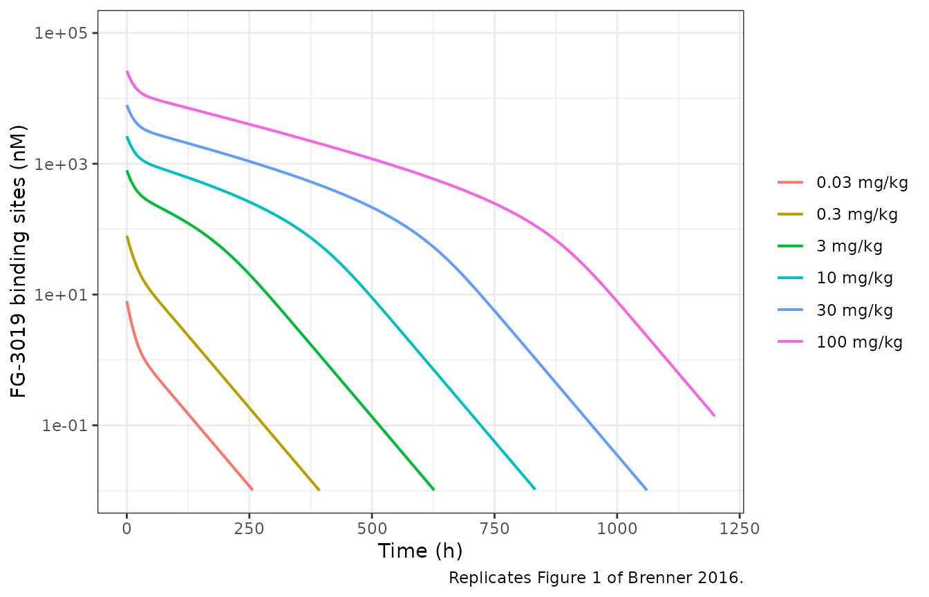
Replicates Figure 1 of Brenner 2016: FG-3019 binding-site concentration after IV bolus doses of 0.03-100 mg/kg.
The characteristic target-mediated shape of the published figure is reproduced: a rapid distribution phase, a concentration-dependent plateau at high dose while the target-mediated route is saturated, and a steeper terminal phase once it is not. As Brenner 2016 notes, the true terminal phase lies well beyond the 504 h sampling window – which is why the published non-compartmental half-lives rise with dose even though a TMDD model has a dose-independent terminal slope.
Replicate Figure 3 – recombinant human CTGF and CTGF-N PK
The human-specific assays do not detect endogenous rat CTGF, so the
paper set W0 = N0 = 0 for these data. Setting both
baselines to (effectively) zero also zeroes the production rates,
because kw and kn are derived from them via
Supplement Eqs. (11)-(12) – exactly the scenario the paper fit.
zero_baselines <- c(bl_ctgf = 1e-12, bl_ctgfn = 1e-12)
tgrid_ctgf <- c(seq(0, 2, by = 0.002), seq(2.05, 24, by = 0.05))

solve_ctgf <- function(amt_nmol, cmt) {
  ev <- rxode2::et(amt = amt_nmol, cmt = cmt, time = 0) |> rxode2::et(tgrid_ctgf)
  s <- as.data.frame(rxode2::rxSolve(mod, ev, params = zero_baselines))
  if (is.null(s$id)) s$id <- 1L
  s
}

fig3 <- bind_rows(
  solve_ctgf(20 * wt_kg, "target_ctgfn") |> mutate(species = "rhCTGF-N", dose = "20 nmol/kg", conc = Cctgf_nw),
  solve_ctgf(40 * wt_kg, "target_ctgfn") |> mutate(species = "rhCTGF-N", dose = "40 nmol/kg", conc = Cctgf_nw),
  solve_ctgf(20 * wt_kg, "target_ctgf")  |> mutate(species = "rhCTGF",   dose = "20 nmol/kg", conc = Cctgf_w),
  solve_ctgf(40 * wt_kg, "target_ctgf")  |> mutate(species = "rhCTGF",   dose = "40 nmol/kg", conc = Cctgf_w)
)

fig3 |>
  filter(conc > 1e-4) |>
  ggplot(aes(time, conc, colour = dose)) +
  geom_line(linewidth = 0.7) +
  facet_wrap(~species, scales = "free") +
  scale_y_log10() +
  labs(x = "Time (h)", y = "Concentration (nM)", colour = NULL,
       caption = "Replicates Figure 3 of Brenner 2016.") +
  theme_bw()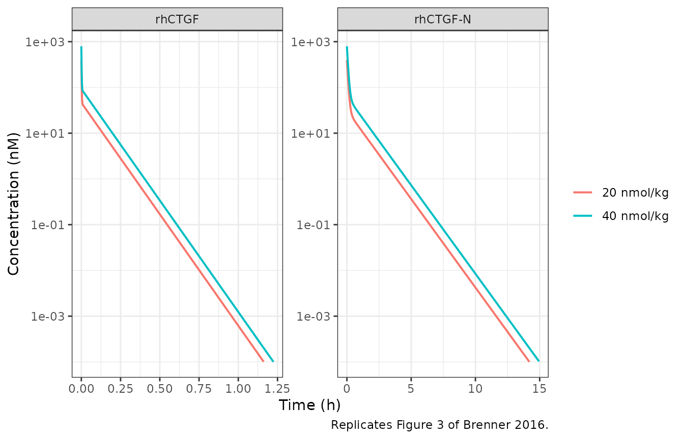
Replicates Figure 3 of Brenner 2016: rhCTGF-N (top) and rhCTGF (bottom) after IV bolus doses of 20 and 40 nmol/kg.
Terminal half-lives of the two CTGF forms
Brenner 2016 reports a 43.5 min terminal half-life for rhCTGF-N and a 3.3 min terminal half-life for intact rhCTGF – the 13-fold difference that motivates the whole model. Both are recovered from the packaged model by regressing the log-linear terminal phase.
tail_slope <- function(df, conc, lo, hi) {
  # Keep conc >= 1e-6 * Cmax: below that the ODE integrator has no relative accuracy left.
  d <- df[df$time >= lo & df$time <= hi & df[[conc]] >= 1e-6 * max(df[[conc]], na.rm = TRUE), ]
  unname(coef(lm(log(d[[conc]]) ~ d$time))[2])
}
sN <- solve_ctgf(20 * wt_kg, "target_ctgfn")
sW <- solve_ctgf(20 * wt_kg, "target_ctgf")

hl <- tibble(
  species = c("rhCTGF-N", "rhCTGF (intact)"),
  model_min = c(log(2) / -tail_slope(sN, "Cctgf_nw", 2, 6) * 60,
                log(2) / -tail_slope(sW, "Cctgf_w", 0.3, 1) * 60),
  paper_min = c(43.5, 3.3)
) |>
  mutate(pct_diff = 100 * (model_min - paper_min) / paper_min)

knitr::kable(hl, digits = 2,
caption = "Terminal half-life of each CTGF form vs Brenner 2016 Results.")| species | model_min | paper_min | pct_diff |
|---|---|---|---|
| rhCTGF-N | 46.66 | 43.5 | 7.27 |
| rhCTGF (intact) | 3.70 | 3.3 | 12.27 |
# Deterministic. The model's true terminal slope vs the paper's NCA estimate on
# sampled mean data; 20% admits that difference, not cohort noise.
stopifnot(all(abs(hl$pct_diff) < 20))
# The 13-fold separation between the two forms is the paper's central claim.
stopifnot(hl$model_min[1] / hl$model_min[2] > 8)
Replicate Figure 2 – endogenous CTGF-N accumulates after FG-3019
Binding FG-3019 raises the apparent molecular weight of CTGF-N above the renal filtration cut-off, so the complex is cleared ~700-fold more slowly than free CTGF-N and the N+W-CTGF signal rises, peaks, and returns to baseline.
fig2 <- lapply(c(10, 30, 100), function(d) solve_fg(d, seq(0, 504, by = 1))) |>
  bind_rows() |>
  mutate(dose = factor(paste0(dose_mgkg, " mg/kg"),
                       levels = paste0(c(10, 30, 100), " mg/kg")))

ggplot(fig2, aes(time, Cctgf_nw, colour = dose)) +
  geom_line(linewidth = 0.7) +
  labs(x = "Time (h)", y = "N+W-CTGF (nM)", colour = NULL,
       caption = "Replicates Figure 2 of Brenner 2016.") +
  theme_bw()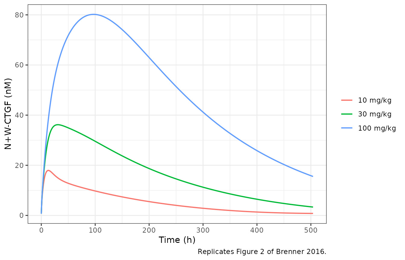
Replicates Figure 2 of Brenner 2016: N+W-CTGF after FG-3019 at 10, 30 and 100 mg/kg.
Brenner 2016’s Figure 2 plots this response on an nM axis (0-160 nM), and the peaks of the published fitted curves read approximately 19, 38 and 86 nM at 10, 30 and 100 mg/kg. The packaged model reproduces them.
fig2_peaks <- fig2 |>
  group_by(dose_mgkg) |>
  summarise(cmax_nM = max(Cctgf_nw), tmax_h = time[which.max(Cctgf_nw)], .groups = "drop") |>
  mutate(fig2_cmax_nM = c(19, 38, 86),
         pct_diff = 100 * (cmax_nM - fig2_cmax_nM) / fig2_cmax_nM)

knitr::kable(fig2_peaks, digits = 1,
caption = "Peak N+W-CTGF vs the fitted curves read off Brenner 2016 Figure 2.")| dose_mgkg | cmax_nM | tmax_h | fig2_cmax_nM | pct_diff |
|---|---|---|---|---|
| 10 | 18.0 | 13 | 19 | -5.5 |
| 30 | 36.2 | 31 | 38 | -4.8 |
| 100 | 80.2 | 97 | 86 | -6.7 |
# Reference values are read off a published figure, so ~15% covers the reading
# error; a mis-transcribed production rate or complex clearance moves these by
# a factor, not by 15%.
stopifnot(all(abs(fig2_peaks$pct_diff) < 15))
# Dose-ordered peak and dose-ordered delay, both stated in the Results text.
stopifnot(
  all(diff(fig2_peaks$cmax_nM) > 0),
  all(diff(fig2_peaks$tmax_h) > 0)
)
Deviation (see Errata). The Results text quotes “Cmax N+W-CTGF concentrations of 32, 77 and 197 ng/ml” for these same three dose groups. Those values cannot be reconciled with Figure 2’s own nM axis under either molecular weight in play (19 kDa for the N-fragment, 38 kDa for intact CTGF): the figure’s peaks correspond to roughly 360, 720 and 1630 ng/mL at 19 kDa. The model reproduces the figure, which is the graphical record of both the data and the fit, so the gate above is written against the figure and the text values are recorded as an internal inconsistency in the source.
Replicate Figure 7 – dose-dependence of target-mediated elimination
This is the paper’s most quantitative single claim and the sharpest available check on the whole structure: at 100 mg/kg, 7.4% of the dose is eliminated by the target-mediated pathway, while at doses at or below 3 mg/kg that pathway is the major route.
ggplot(balance, aes(dose_mgkg, pct_target_mediated)) +
  geom_line(linewidth = 0.7) + geom_point() +
  geom_hline(yintercept = 50, linetype = "dashed", colour = "grey50") +
  scale_x_log10() +
  labs(x = "FG-3019 dose (mg/kg)", y = "Target-mediated elimination (%)",
       caption = "Replicates Figure 7 of Brenner 2016.") +
  theme_bw()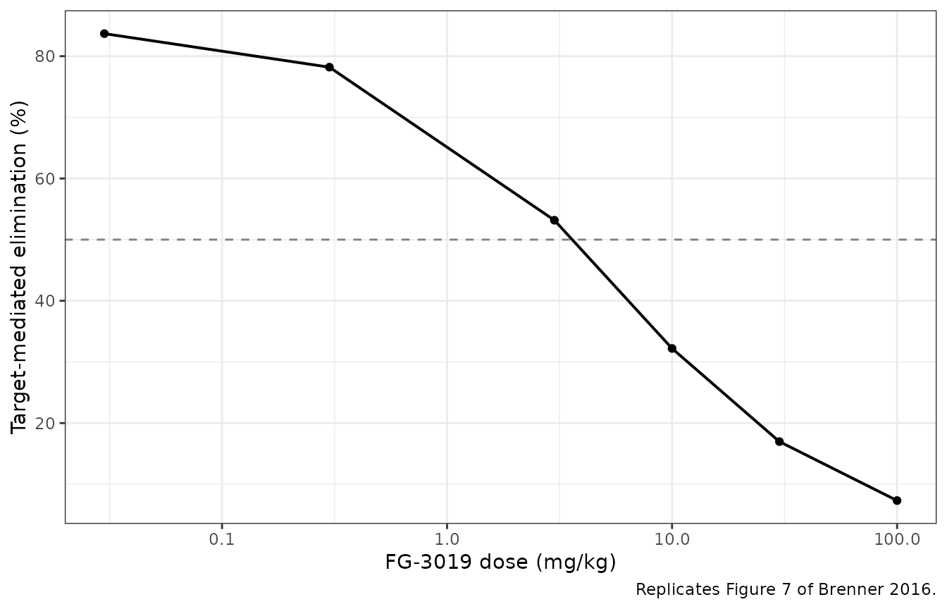
Replicates Figure 7 of Brenner 2016: percent of the FG-3019 dose eliminated by the target-mediated pathway.
pct_100 <- balance$pct_target_mediated[balance$dose_mgkg == 100]
pct_le3 <- balance$pct_target_mediated[balance$dose_mgkg <= 3]
c(model_pct_at_100mgkg = pct_100, paper_pct_at_100mgkg = 7.4)
#> model_pct_at_100mgkg paper_pct_at_100mgkg
#>             7.327112             7.400000

# Deterministic and directly quoted in the Results; 1 percentage point is tight
# but comfortable (realised difference ~0.1).
stopifnot(abs(pct_100 - 7.4) < 1)
# "For doses at or below 3 mg/kg, target-mediated clearance is the major pathway"
stopifnot(all(pct_le3 > 50))
# Monotone decreasing with dose, as Figure 7 shows.
stopifnot(all(diff(balance$pct_target_mediated) < 0))
PKNCA validation against Table S1
Table S1 of the supplement reports non-compartmental parameters for each FG-3019 dose group. To compare like with like, the model is sampled on a schedule matching the study design (one pre-dose plus 12 post-dose points to 504 h) and analysed with PKNCA in the paper’s units (ug/mL, days).
# Study-design sampling schedule (Brenner 2016 Methods: 12 post-dose points to 504 h).
sample_h <- c(0, 0.083, 0.5, 1, 6, 24, 48, 72, 120, 168, 240, 336, 504)

nca_sim <- lapply(doses, function(d) solve_fg(d, sample_h)) |>
  bind_rows() |>
  transmute(
    id        = as.integer(factor(dose_mgkg, levels = doses)),
    treatment = factor(paste0(dose_mgkg, " mg/kg"), levels = paste0(doses, " mg/kg")),
    time      = time / 24,                       # days
    Cc        = Cc * ug_per_mL_per_nM            # ug/mL
  )

# Only !is.na(); dropping time == 0 would remove PKNCA's AUC anchor.
nca_sim <- nca_sim |> filter(!is.na(Cc)) |>
  # Per subject, keep Cc >= 1e-6 * Cmax after the peak: below that the ODE integrator has no relative accuracy left.
  group_by(id) |>
  filter(time <= time[which.max(Cc)] | Cc >= 1e-6 * max(Cc)) |>
  ungroup()
stopifnot(nrow(nca_sim) > 0, any(nca_sim$time == 0))

dose_df <- tibble(
  id        = as.integer(factor(doses, levels = doses)),
  treatment = factor(paste0(doses, " mg/kg"), levels = paste0(doses, " mg/kg")),
  time      = 0,
  amt       = doses * wt_kg                      # mg administered
)

conc_obj <- PKNCA::PKNCAconc(as.data.frame(nca_sim), Cc ~ time | treatment + id)
dose_obj <- PKNCA::PKNCAdose(as.data.frame(dose_df), amt ~ time | treatment + id,
                             route = "intravascular")

intervals <- data.frame(
  start = 0, end = Inf,
  cmax = TRUE, tmax = TRUE, aucinf.obs = TRUE, half.life = TRUE, cl.obs = TRUE
)

nca_res <- PKNCA::pk.nca(PKNCA::PKNCAdata(conc_obj, dose_obj, intervals = intervals))
published <- tibble::tribble(
  ~treatment,     ~cmax,  ~aucinf.obs, ~half.life,
  "0.03 mg/kg",   0.453,  0.34,        1.36,
  "0.3 mg/kg",    5.75,   7.50,        1.63,
  "3 mg/kg",      63.3,   207,         1.70,
  "10 mg/kg",     292,    611,         2.62,
  "30 mg/kg",     828,    2490,        3.92,
  "100 mg/kg",    2665,   11300,       7.31
)

cmp <- nlmixr2lib::ncaComparisonTable(
  simulated = nca_res,
  reference = published,
  by        = "treatment",
  units     = c(cmax = "ug/mL", aucinf.obs = "day*ug/mL", half.life = "day"),
  tolerance_pct = 20
)

knitr::kable(cmp, caption = "Simulated vs Brenner 2016 Table S1. * differs by >20%.")| NCA parameter | treatment | Reference | Simulated | % diff |
|---|---|---|---|---|
| Cmax (ug/mL) | 0.03 mg/kg | 0.453 | 0.595 | +31.4%* |
| Cmax (ug/mL) | 0.3 mg/kg | 5.75 | 5.95 | +3.5% |
| Cmax (ug/mL) | 3 mg/kg | 63.3 | 59.5 | -6.0% |
| Cmax (ug/mL) | 10 mg/kg | 292 | 198 | -32.1%* |
| Cmax (ug/mL) | 30 mg/kg | 828 | 595 | -28.1%* |
| Cmax (ug/mL) | 100 mg/kg | 2660 | 1980 | -25.5%* |
| AUC0-∞ (obs) (day*ug/mL) | 0.03 mg/kg | 0.34 | 0.475 | +39.8%* |
| AUC0-∞ (obs) (day*ug/mL) | 0.3 mg/kg | 7.5 | 6.29 | -16.1% |
| AUC0-∞ (obs) (day*ug/mL) | 3 mg/kg | 207 | 134 | -35.5%* |
| AUC0-∞ (obs) (day*ug/mL) | 10 mg/kg | 611 | 642 | +5.0% |
| AUC0-∞ (obs) (day*ug/mL) | 30 mg/kg | 2490 | 2420 | -2.9% |
| AUC0-∞ (obs) (day*ug/mL) | 100 mg/kg | 11300 | 9030 | -20.1%* |
| t½ (day) | 0.03 mg/kg | 1.36 | 1.42 | +4.1% |
| t½ (day) | 0.3 mg/kg | 1.63 | 1.42 | -13.0% |
| t½ (day) | 3 mg/kg | 1.7 | 1.44 | -15.2% |
| t½ (day) | 10 mg/kg | 2.62 | 2.12 | -19.1% |
| t½ (day) | 30 mg/kg | 3.92 | 4.96 | +26.4%* |
| t½ (day) | 100 mg/kg | 7.31 | 6.09 | -16.7% |
The comparison is informative but is not a like-for-like test of the model, for a reason the paper states itself: “sample collection from animals administered high doses of FG-3019 was terminated too soon to establish the true terminal elimination rates. This failure to collect samples at sufficiently late time points explains the apparent dose-dependence of the experimentally determined half-lives.” Table S1’s half-lives and extrapolated AUCs therefore carry a dose-dependent truncation bias that the model, which has a dose-independent true terminal slope, does not share. The rows are expected to diverge at the high doses and are reported rather than gated.
What is gated is the non-linearity that the paper drew its conclusion from: clearance must fall, and dose-normalised exposure must rise, monotonically with dose.
nca_tab <- as.data.frame(nca_res) |>
  filter(PPTESTCD %in% c("cl.obs", "aucinf.obs")) |>
  select(treatment, PPTESTCD, PPORRES) |>
  pivot_wider(names_from = PPTESTCD, values_from = PPORRES) |>
  mutate(
    dose_mgkg   = doses[match(treatment, paste0(doses, " mg/kg"))],
    cl_mL_day_kg = cl.obs * 1000 / wt_kg,
    auc_per_dose = aucinf.obs / dose_mgkg
  ) |>
  arrange(dose_mgkg)

nca_tab |>
  select(treatment, cl_mL_day_kg, auc_per_dose) |>
  dplyr::rename(
    "Dose group"                          = treatment,
    "CL (mL/day/kg)"                      = cl_mL_day_kg,
    "AUCinf/Dose (day*ug/mL per mg/kg)"   = auc_per_dose
  ) |>
  knitr::kable(digits = 1,
caption = "Model non-linearity: CL falls and dose-normalised AUC rises with dose.")| Dose group | CL (mL/day/kg) | AUCinf/Dose (day*ug/mL per mg/kg) |
|---|---|---|
| 0.03 mg/kg | 63.1 | 15.8 |
| 0.3 mg/kg | 47.7 | 21.0 |
| 3 mg/kg | 22.5 | 44.5 |
| 10 mg/kg | 15.6 | 64.2 |
| 30 mg/kg | 12.4 | 80.6 |
| 100 mg/kg | 11.1 | 90.3 |
# Deterministic solves, no cohort: assert the monotonicity directly.
stopifnot(
  all(diff(nca_tab$cl_mL_day_kg) < 0),
  all(diff(nca_tab$auc_per_dose) > 0)
)
# Brenner 2016 Results: CL falls from 90.6 to 8.9 mL/kg/day, a ~10-fold span.
stopifnot(
  nca_tab$cl_mL_day_kg[1] / nca_tab$cl_mL_day_kg[nrow(nca_tab)] > 4
)
Assumptions and deviations
-
No IIV and no residual error. Brenner 2016 fit
mean data by maximum likelihood in ADAPT 5 and reports only
estimation precision (CV%) in Table I. No between-animal variance and no
residual-error model are published, so none is encoded; the model is a
typical-value mechanistic simulator. The CV% values are preserved in the
ini()source-trace comments. -
Constrained parameters are derived, not duplicated.
Table I footnotes a-d record equality constraints
(
CLN = CLW;CLAb = CLAbW = CLAbN;CLdAbN = CLdAb;CLAbWT = CLWT) and the Methods addVAbWT = VWTandVAbNT = VAbT. These are computed inmodel()from the free parameters so the constraints cannot drift apart. -
CLAbWtypographical inconsistency in Table I. Table I printsCLAbW = 0.0001331 L/hcarrying footnote b, but footnote b itself statesCLAb = CLAbW = CLAbN, and bothCLAbandCLAbNare printed as0.0001321 L/h. The footnote is the constraint actually imposed during the fit and two of the three printed values agree with it, so0.0001321is used for all three and the printed0.0001331is treated as a typesetting error. The effect either way is below 1%. - Figure 2 vs the Results text. The Results text quotes peak N+W-CTGF concentrations of “32, 77 and 197 ng/ml” at 10, 30 and 100 mg/kg. These are irreconcilable with Figure 2’s own nM axis (peaks near 19, 38 and 86 nM, i.e. roughly 360, 720 and 1630 ng/mL at the N-fragment’s 19 kDa). The packaged model reproduces the figure to within about 6%; the figure is used as the validation target and the text values are recorded here as an internal inconsistency in the source. No parameter was adjusted.
- Table S1 NCA is not gated. See the PKNCA section: the published non-compartmental parameters carry a dose-dependent terminal-phase truncation bias that the authors describe explicitly. The comparison table is rendered for transparency; the gated claim is the direction and magnitude of the non-linearity.
- Experiments excluded by the authors. The CTGF and RAP co-administration studies (Figs. 4-5) were not part of the fit – the model treats FG-3019 as monovalent 75 kDa, whereas co-dosed rhCTGF forms 2:1 complexes with the bivalent antibody, and rat RAP kinetics were unavailable. They are therefore not reproduced here.
-
Fitting the human-CTGF experiments. For Figure 3
the paper set
W0 = N0 = 0because the human-specific assays do not detect endogenous rat CTGF. This vignette reproduces that by setting both baselines to 1e-12 nM, which also zeroes the derived production rateskwandkn. - Species. All parameters are rat (Sprague-Dawley) values normalised to a 0.3 kg animal. The paper notes non-linear FG-3019 PK was also seen in monkeys and humans, but reports no parameters for those species.
- Every parameter value comes from the paper’s Table I or its Electronic Supplementary Material. No value was taken from any other source, digitised from a figure, or supplied by correspondence.