Cefiderocol in pneumonia, BSI/sepsis and cUTI (Kawaguchi 2021)
Source:vignettes/articles/Kawaguchi_2021_cefiderocol.Rmd
Kawaguchi_2021_cefiderocol.RmdModel and source
Kawaguchi 2021 updates the same group’s earlier cefiderocol
population PK analysis (Kawaguchi_2018_cefiderocol_clcr and
its siblings) with the two phase 3 studies, APEKS-NP (pneumonia) and
CREDIBLE-CR (pneumonia, bloodstream infection/sepsis or complicated
urinary tract infection caused by carbapenem-resistant pathogens). The
structure is unchanged – three compartments, intravenous infusion,
first-order elimination – but the covariate model is new: clearance now
follows Cockcroft-Gault creatinine clearance only up to 150 mL/min, each
infection site carries its own factor on clearance, and serum albumin
enters the central volume.
mod <- rxode2::rxode(readModelDb("Kawaguchi_2021_cefiderocol"))
#> ℹ parameter labels from comments will be replaced by 'label()'
cat(mod$reference)
#> Kawaguchi N, Katsube T, Echols R, Wajima T. Population pharmacokinetic and pharmacokinetic/pharmacodynamic analyses of cefiderocol, a parenteral siderophore cephalosporin, in patients with pneumonia, bloodstream infection/sepsis, or complicated urinary tract infection. Antimicrob Agents Chemother. 2021;65(3):e01437-20. doi:10.1128/AAC.01437-20- Article: https://doi.org/10.1128/AAC.01437-20
- Supplement (Tables S1-S3 including the final NONMEM control stream, Figures S1-S5): available from the article page.
Population
pop <- mod$population
str(pop[c("n_subjects", "n_studies", "n_observations", "age_range",
          "weight_range", "sex_female_pct")])
#> List of 6
#>  $ n_subjects    : int 516
#>  $ n_studies     : int 5
#>  $ n_observations: int 3427
#>  $ age_range     : chr "18-93 years (per-study medians 36.0 phase 1, 65.0 APEKS-cUTI, 68.0 APEKS-NP, 67.5 CREDIBLE-CR)"
#>  $ weight_range  : chr "25.0-156.0 kg (per-study medians 68.4-76.4 kg)"
#>  $ sex_female_pct: num 40.1
The analysis pooled 3427 plasma concentrations from 516 subjects in five studies (Table 1, Table S1): 91 subjects without infection from two phase 1 studies (healthy volunteers and a renal-impairment study), 238 patients with cUTI or acute uncomplicated pyelonephritis from the phase 2 APEKS-cUTI study, 115 pneumonia patients from APEKS-NP, and 72 patients from CREDIBLE-CR (31 pneumonia, 20 BSI/sepsis, 21 cUTI). Body weight ranged 25-156 kg and Cockcroft-Gault creatinine clearance 4-306 mL/min; the phase 3 patients were markedly hypoalbuminaemic (median 2.7-3.0 g/dL against 4.2 g/dL in the earlier studies). Hemodialysis patients were excluded. About 40% of subjects were female.
Source trace
Every value below comes from Table 2 of the article (final model column) or the final NONMEM control stream printed as Table S2. The two agree everywhere.
| Quantity | Value | Source |
|---|---|---|
| Structure: 3-compartment IV, first-order elimination | ADVAN11 TRANS4 | Results; Table S2 |
| CL (uninfected, CRCL 83.0 mL/min) | 4.04 L/h | Table 2; footnote b |
| V1 (uninfected, 72.6 kg, albumin 3.9 g/dL) | 7.78 L | Table 2; footnote b |
| Q2 | 6.19 L/h | Table 2 |
| V2 (72.6 kg) | 5.77 L | Table 2; footnote b |
| Q3 | 0.127 L/h | Table 2 |
| V3 | 0.798 L | Table 2 |
| CRCL exponent on CL, CRCL capped at 150 mL/min | 0.682 | Table 2; footnote b; Table S2 CLCR1
|
| Weight exponent on V1 and V2 (shared) | 0.580 | Table 2; Table S2 WT1
|
| Pneumonia factor on CL | 0.981 | Table 2; Table S2 PT14
|
| BSI/sepsis factor on CL | 1.08 | Table 2; Table S2 PT13
|
| cUTI (CREDIBLE-CR) factor on CL | 0.872 | Table 2; Table S2 PT12
|
| cUTI/AUP (APEKS-cUTI) factor on CL | 1.27 | Table 2; Table S2 PT11
|
| Albumin exponent on V1, centred at 3.9 g/dL | -0.617 | Table 2; footnote b; Table S2 ALB2
|
| Any-infection factor on V1 | 1.39 | Table 2; Table S2 PTV
|
| IIV CL, V1, V2 (CV%) | 37.5, 56.9, 33.6 | Table 2 |
| Covariances CL-V1, CL-V2, V1-V2 | 0.0886, 0.0792, 0.150 | Table 2 (footnotes c-e give R) |
| Proportional residual error | 20.5% | Table 2; Table S2 W = IPRED*THETA(7),
$SIGMA 1 FIX
|
| Unbound fraction for fT>MIC | 0.422 | Materials and Methods |
The omega scale
Table 2 prints IIV as a percent CV together with the three
covariances and their correlation coefficients. That over-determines the
scale. If the variance is (CV/100)^2, the implied
covariance R * sd_a * sd_b must reproduce the printed
covariance; under the log-normal reading
sd = sqrt(log(1 + CV^2)) it would be about 10% smaller.
cv <- c(CL = 0.375, V1 = 0.569, V2 = 0.336)
printed <- data.frame(
  pair = c("CL-V1", "CL-V2", "V1-V2"),
  a = c("CL", "CL", "V1"), b = c("V1", "V2", "V2"),
  cov = c(0.0886, 0.0792, 0.150),
  R = c(0.415, 0.629, 0.784)
)
sd_cv <- cv
sd_ln <- sqrt(log(1 + cv^2))
printed$cov_if_cv <- printed$R * sd_cv[printed$a] * sd_cv[printed$b]
printed$cov_if_lognormal <- printed$R * sd_ln[printed$a] * sd_ln[printed$b]
knitr::kable(printed[, c("pair", "cov", "cov_if_cv", "cov_if_lognormal")],
digits = 4)| pair | cov | cov_if_cv | cov_if_lognormal |
|---|---|---|---|
| CL-V1 | 0.0886 | 0.0886 | 0.0797 |
| CL-V2 | 0.0792 | 0.0793 | 0.0746 |
| V1-V2 | 0.1500 | 0.1499 | 0.1358 |
stopifnot(
  all(abs(printed$cov_if_cv / printed$cov - 1) < 0.005),
  all(abs(printed$cov_if_lognormal / printed$cov - 1) > 0.05)
)

# And the packaged omega matrix carries exactly those values.
om <- mod$omega
stopifnot(
  all(abs(diag(om) - cv^2) < 1e-12),
  abs(om["etalcl", "etalvc"] - 0.0886) < 1e-12,
  abs(om["etalcl", "etalvp"] - 0.0792) < 1e-12,
  abs(om["etalvc", "etalvp"] - 0.150) < 1e-12
)
Deterministic verification
m0 <- suppressMessages(rxode2::zeroRe(mod))

# rxode2 warns when a zero-omega model is solved for many subjects; that is
# intended here, so only that one warning is muffled.
solve_quiet <- function(model, events, ...) {
  withCallingHandlers(
    as.data.frame(rxode2::rxSolve(model, events, returnType = "data.frame", ...)),
    warning = function(w) {
      if (grepl("without 'omega'", conditionMessage(w))) {
        invokeRestart("muffleWarning")
      }
    }
  )
}

cov_defaults <- c(DIS_PNEUMONIA = 0, DIS_BACTEREMIA = 0, DIS_CUTI = 0,
                  STUDY_CEFIDEROCOL_PHASE2 = 0)
The Table 2 footnote equations, reproduced exactly
Footnote b of Table 2 prints the full covariate equations. The packaged model must reproduce them to machine precision over a grid that crosses the 150 mL/min clearance cap, spans body weight and albumin, and visits every infection site.
sites <- data.frame(
  site = c("none", "pneumonia", "BSI/sepsis", "cUTI (CREDIBLE-CR)", "cUTI/AUP (APEKS-cUTI)"),
  DIS_PNEUMONIA = c(0, 1, 0, 0, 0),
  DIS_BACTEREMIA = c(0, 0, 1, 0, 0),
  DIS_CUTI = c(0, 0, 0, 1, 1),
  STUDY_CEFIDEROCOL_PHASE2 = c(0, 0, 0, 0, 1),
  f_cl = c(1, 0.981, 1.08, 0.872, 1.27),
  f_v1 = c(1, 1.39, 1.39, 1.39, 1.39)
)
grid <- tidyr::expand_grid(
  CRCL = c(10, 83, 149, 150, 151, 300),
  WT = c(40, 72.6, 120),
  ALB = c(15, 39, 50),          # g/L
  sites
)
grid$id <- seq_len(nrow(grid))
ev_grid <- grid |>
  select(id, CRCL, WT, ALB, DIS_PNEUMONIA, DIS_BACTEREMIA, DIS_CUTI,
         STUDY_CEFIDEROCOL_PHASE2) |>
  mutate(time = 1, amt = 0, evid = 0L, cmt = "central")
typ <- solve_quiet(m0, ev_grid) |>
  select(id, cl, vc, vp)
#> ℹ omega/sigma items treated as zero: 'etalcl', 'etalvc', 'etalvp'
chk <- grid |>
  inner_join(typ, by = "id") |>
  mutate(
    cl_paper = 4.04 * (pmin(CRCL, 150) / 83.0)^0.682 * f_cl,
    v1_paper = 7.78 * (WT / 72.6)^0.580 * ((ALB / 10) / 3.9)^-0.617 * f_v1,
    v2_paper = 5.77 * (WT / 72.6)^0.580
  )
c(cl = max(abs(chk$cl / chk$cl_paper - 1)),
  v1 = max(abs(chk$vc / chk$v1_paper - 1)),
  v2 = max(abs(chk$vp / chk$v2_paper - 1)))
#>           cl           v1           v2
#> 1.332268e-15 5.551115e-16 1.776357e-15
stopifnot(
  nrow(chk) == nrow(grid),
  all(abs(chk$cl / chk$cl_paper - 1) < 1e-10),
  all(abs(chk$vc / chk$v1_paper - 1) < 1e-10),
  all(abs(chk$vp / chk$v2_paper - 1) < 1e-10)
)
The paper’s quoted percentages
The Results and Discussion state that CL in APEKS-cUTI patients was “27% higher than that in subjects without infection” and that V1 in infected patients was “39% higher”. Clearance must also be flat above 150 mL/min.
at <- function(site_name, crcl = 83) {
  chk[chk$site == site_name & chk$CRCL == crcl & chk$WT == 72.6 & chk$ALB == 39, ]
}
ratio_cl_cuti <- at("cUTI/AUP (APEKS-cUTI)")$cl / at("none")$cl
ratio_v1_inf <- at("pneumonia")$vc / at("none")$vc
flat <- at("none", 300)$cl / at("none", 150)$cl
c(cl_cuti = ratio_cl_cuti, v1_infected = ratio_v1_inf, cl_300_vs_150 = flat)
#>       cl_cuti   v1_infected cl_300_vs_150
#>          1.27          1.39          1.00
stopifnot(
  abs(ratio_cl_cuti - 1.27) < 1e-10,
  abs(ratio_v1_inf - 1.39) < 1e-10,
  abs(flat - 1) < 1e-12,
  at("none", 151)$cl == at("none", 150)$cl,
  at("none", 149)$cl < at("none", 150)$cl
)
The infusion is an infusion
A single 2 g dose infused over 3 h in a typical pneumonia patient must peak at the end of the infusion, not at time zero.
ev_single <- data.frame(
  id = 1, time = c(0, seq(0.25, 48, by = 0.25)),
  amt = c(2000, rep(0, 192)), dur = c(3, rep(NA, 192)),
  evid = c(1L, rep(0L, 192)), cmt = "central",
  CRCL = 83, WT = 72.6, ALB = 28, DIS_PNEUMONIA = 1, DIS_BACTEREMIA = 0,
  DIS_CUTI = 0, STUDY_CEFIDEROCOL_PHASE2 = 0
)
single <- solve_quiet(m0, ev_single)
#> ℹ omega/sigma items treated as zero: 'etalcl', 'etalvc', 'etalvp'
tmax <- single$time[which.max(single$Cc)]
tmax
#> [1] 3
stopifnot(tmax == 3)
Virtual cohort
The paper’s Monte-Carlo simulation (Tables 3-4 and Figure 4 captions;
Materials and Methods) generated, for each infection site, patients in
six renal-function groups defined by Cockcroft-Gault CRCL: augmented
(120 to 150 and above 150 mL/min, half each), normal (90 to <120),
mild (60 to <90), moderate (30 to <60), severe (15 to <30) and
ESRD (5 to <15). Body weight was log-normal with mean 72.6 kg and CV
30%, albumin log-normal with mean 2.8 g/dL and CV 30%. The cUTI
simulations used the CREDIBLE-CR coefficient
(STUDY_CEFIDEROCOL_PHASE2 = 0).
The paper simulated 1,000 patients per scenario; this vignette uses 200. Both the covariates and the random effects are drawn with base R, which is reproducible across R builds, and the model is then solved with its random effects zeroed and the drawn etas supplied as data columns. This keeps every number below identical across rxode2 versions.
set.seed(20210217)
n_per_arm <- 200
regimens <- data.frame(
  renal = c("Augmented", "Normal", "Mild", "Moderate", "Severe", "ESRD"),
  crcl_lo = c(120, 90, 60, 30, 15, 5),
  crcl_hi = c(150, 120, 90, 60, 30, 15),
  dose_mg = c(2000, 2000, 2000, 1500, 1000, 750),
  tau = c(6, 8, 8, 8, 8, 12)
)
infection_sites <- c("Pneumonia", "BSI/sepsis", "cUTI")
sd_log <- function(cv) sqrt(log(1 + cv^2))
chol_om <- chol(mod$omega)

arms <- list()
for (s in infection_sites) {
  for (g in seq_len(nrow(regimens))) {
    r <- regimens[g, ]
    crcl <- if (r$renal == "Augmented") {
      # Half 120 to <150, half above 150. CL is flat above 150 mL/min, so the
      # upper bound of 200 mL/min only affects the covariate column.
      c(runif(n_per_arm / 2, 120, 150), runif(n_per_arm / 2, 150, 200))
    } else {
      runif(n_per_arm, r$crcl_lo, r$crcl_hi)
    }
    eta <- matrix(rnorm(3 * n_per_arm), n_per_arm) %*% chol_om
    arms[[length(arms) + 1]] <- data.frame(
      site = s, renal = r$renal, dose_mg = r$dose_mg, tau = r$tau,
      CRCL = crcl,
      WT = rlnorm(n_per_arm, log(72.6) - sd_log(0.3)^2 / 2, sd_log(0.3)),
      ALB = 10 * rlnorm(n_per_arm, log(2.8) - sd_log(0.3)^2 / 2, sd_log(0.3)),
      DIS_PNEUMONIA = as.integer(s == "Pneumonia"),
      DIS_BACTEREMIA = as.integer(s == "BSI/sepsis"),
      DIS_CUTI = as.integer(s == "cUTI"),
      STUDY_CEFIDEROCOL_PHASE2 = 0L,
      etalcl = eta[, 1], etalvc = eta[, 2], etalvp = eta[, 3]
    )
  }
}
cohort <- dplyr::bind_rows(arms)
cohort$id <- seq_len(nrow(cohort))
cohort$treatment <- paste(cohort$site, cohort$renal, sep = ": ")

cohort |>
  group_by(site) |>
  summarise(n = n(), WT_mean = mean(WT), ALB_mean_gdL = mean(ALB) / 10,
            .groups = "drop") |>
knitr::kable(digits = 2)| site | n | WT_mean | ALB_mean_gdL |
|---|---|---|---|
| BSI/sepsis | 1200 | 73.15 | 2.78 |
| Pneumonia | 1200 | 72.94 | 2.76 |
| cUTI | 1200 | 72.54 | 2.79 |
Simulation
Each subject is simulated over one steady-state dosing interval (3 h
infusion, ss = 1), observed every 0.05 h.
cov_cols <- c("CRCL", "WT", "ALB", "DIS_PNEUMONIA", "DIS_BACTEREMIA", "DIS_CUTI",
              "STUDY_CEFIDEROCOL_PHASE2", "etalcl", "etalvc", "etalvp")
dose_rows <- cohort |>
  transmute(id, time = 0, amt = dose_mg, dur = 3, ii = tau, ss = 1L,
            evid = 1L, cmt = "central") |>
  bind_cols(cohort[, cov_cols])
obs_rows <- cohort |>
  select(id, tau, all_of(cov_cols)) |>
  reframe(time = seq(0, tau, by = 0.05), .by = c(id, tau, all_of(cov_cols))) |>
  mutate(amt = 0, dur = NA_real_, ii = 0, ss = 0L, evid = 0L, cmt = "central") |>
  select(-tau)
events <- bind_rows(dose_rows, obs_rows) |>
  arrange(id, time, desc(evid))

# maxsteps: the lsoda step budget is charged across the steady-state search.
sim <- solve_quiet(m0, events, maxsteps = 1e6) |>
  select(id, time, Cc, cl) |>
  inner_join(cohort |> select(id, site, renal, treatment, tau, dose_mg), by = "id")
#> ℹ omega/sigma items treated as zero: 'etalcl', 'etalvc', 'etalvp'
stopifnot(!anyNA(sim$Cc), all(sim$Cc > 0))
Typical profiles by infection site
typ_ev <- sites |>
  filter(site != "cUTI/AUP (APEKS-cUTI)") |>
  mutate(id = row_number(), CRCL = 83, WT = 72.6, ALB = 28)
typ_ev <- typ_ev |>
  select(-f_cl, -f_v1) |>
  tidyr::crossing(time = seq(0, 48, by = 0.1)) |>
  mutate(amt = 0, dur = NA_real_, ii = 0, addl = 0L, evid = 0L, cmt = "central") |>
  bind_rows(
    typ_ev |>
      select(-f_cl, -f_v1) |>
      mutate(time = 0, amt = 2000, dur = 3, ii = 8, addl = 5L, evid = 1L,
             cmt = "central")
  ) |>
  arrange(id, time, desc(evid))
typ_sim <- solve_quiet(m0, typ_ev, keep = "site")
#> ℹ omega/sigma items treated as zero: 'etalcl', 'etalvc', 'etalvp'
ggplot(typ_sim, aes(time, Cc, colour = site)) +
  geom_line() +
  scale_y_log10() +
  labs(x = "Time (h)", y = "Total cefiderocol (ug/mL)", colour = NULL,
       caption = paste("Typical patient, CRCL 83 mL/min, 72.6 kg, albumin",
                       "2.8 g/dL, 2 g q8h over 3 h.")) +
  theme_bw()
#> Warning in scale_y_log10(): log-10 transformation introduced infinite values.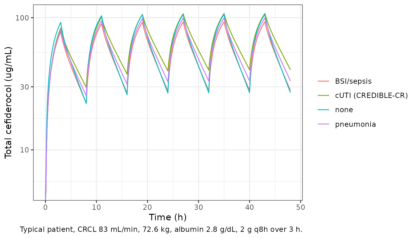
Replicate published tables
Tables 3 and 4 – probability of target attainment
The free concentration is 0.422 * Cc (Materials and
Methods). The percentage of the dosing interval with free concentration
above the MIC (%fT>MIC) is the fraction of the 0.05 h grid over
[0, tau) above the MIC; 100% fT>MIC is equivalent to a
free trough above the MIC.
mics <- c(0.25, 0.5, 1, 2, 4, 8, 16)
ft <- sim |>
  filter(time < tau) |>
  mutate(Cfree = 0.422 * Cc) |>
  tidyr::crossing(mic = mics) |>
  group_by(id, site, renal, mic) |>
  summarise(ft = mean(Cfree > mic), .groups = "drop")
pta_sim <- ft |>
  group_by(site, renal, mic) |>
  summarise(pta75 = 100 * mean(ft >= 0.75), pta100 = 100 * mean(ft >= 1),
            .groups = "drop")

# Kawaguchi 2021 Table 3 (75% fT>MIC) and Table 4 (100% fT>MIC).
pta_row <- function(site, renal, target, v) {
  data.frame(site = site, renal = renal, target = target, mic = mics, paper = v)
}
paper <- rbind(
  pta_row("Pneumonia", "Augmented", 75, c(100, 100, 100, 100, 99.7, 94.5, 60.4)),
  pta_row("Pneumonia", "Normal", 75, c(100, 100, 100, 99.9, 98.9, 87.1, 43.4)),
  pta_row("Pneumonia", "Mild", 75, c(100, 100, 100, 100, 99.8, 97.0, 69.7)),
  pta_row("Pneumonia", "Moderate", 75, c(100, 100, 100, 100, 99.9, 98.7, 83.3)),
  pta_row("Pneumonia", "Severe", 75, c(100, 100, 100, 100, 100, 99.9, 90.7)),
  pta_row("Pneumonia", "ESRD", 75, c(100, 100, 100, 100, 100, 99.6, 86.3)),
  pta_row("BSI/sepsis", "Augmented", 75, c(100, 100, 100, 100, 99.4, 91.3, 49.6)),
  pta_row("BSI/sepsis", "Normal", 75, c(100, 100, 100, 99.9, 97.3, 80.6, 32.6)),
  pta_row("BSI/sepsis", "Mild", 75, c(100, 100, 100, 99.9, 99.6, 94.4, 57.7)),
  pta_row("BSI/sepsis", "Moderate", 75, c(100, 100, 100, 100, 99.9, 98.0, 74.8)),
  pta_row("BSI/sepsis", "Severe", 75, c(100, 100, 100, 100, 100, 99.8, 84.8)),
  pta_row("BSI/sepsis", "ESRD", 75, c(100, 100, 100, 100, 100, 99.2, 79.2)),
  pta_row("cUTI", "Augmented", 75, c(100, 100, 100, 100, 99.9, 96.9, 73.3)),
  pta_row("cUTI", "Normal", 75, c(100, 100, 100, 100, 99.6, 93.6, 56.3)),
  pta_row("cUTI", "Mild", 75, c(100, 100, 100, 100, 99.8, 98.4, 81.2)),
  pta_row("cUTI", "Moderate", 75, c(100, 100, 100, 100, 100, 99.6, 90.4)),
  pta_row("cUTI", "Severe", 75, c(100, 100, 100, 100, 100, 100, 95.9)),
  pta_row("cUTI", "ESRD", 75, c(100, 100, 100, 100, 100, 100, 91.6)),
  pta_row("Pneumonia", "Augmented", 100, c(100, 100, 100, 99.7, 95.9, 79.8, 37.0)),
  pta_row("Pneumonia", "Normal", 100, c(100, 100, 99.9, 98.3, 91.2, 64.6, 23.2)),
  pta_row("Pneumonia", "Mild", 100, c(100, 100, 99.9, 99.7, 98.2, 85.9, 46.4)),
  pta_row("Pneumonia", "Moderate", 100, c(100, 100, 100, 100, 99.5, 94.8, 66.7)),
  pta_row("Pneumonia", "Severe", 100, c(100, 100, 100, 100, 100, 99.5, 81.8)),
  pta_row("Pneumonia", "ESRD", 100, c(100, 100, 100, 100, 100, 98.3, 77.1)),
  pta_row("BSI/sepsis", "Augmented", 100, c(100, 100, 100, 99.4, 93.6, 71.6, 28.5)),
  pta_row("BSI/sepsis", "Normal", 100, c(100, 99.9, 99.5, 96.2, 85.8, 54.0, 14.1)),
  pta_row("BSI/sepsis", "Mild", 100, c(100, 100, 99.8, 99.4, 96.0, 78.0, 36.1)),
  pta_row("BSI/sepsis", "Moderate", 100, c(100, 100, 100, 99.9, 98.7, 91.2, 55.8)),
  pta_row("BSI/sepsis", "Severe", 100, c(100, 100, 100, 100, 100, 98.3, 74.7)),
  pta_row("BSI/sepsis", "ESRD", 100, c(100, 100, 100, 100, 100, 96.8, 68.0)),
  pta_row("cUTI", "Augmented", 100, c(100, 100, 100, 100, 98.0, 88.3, 51.1)),
  pta_row("cUTI", "Normal", 100, c(100, 100, 99.9, 99.4, 95.1, 77.6, 34.3)),
  pta_row("cUTI", "Mild", 100, c(100, 100, 100, 99.8, 98.9, 93.2, 59.4)),
  pta_row("cUTI", "Moderate", 100, c(100, 100, 100, 100, 99.8, 97.7, 79.1)),
  pta_row("cUTI", "Severe", 100, c(100, 100, 100, 100, 100, 99.7, 90.1)),
  pta_row("cUTI", "ESRD", 100, c(100, 100, 100, 100, 100, 99.4, 85.7))
)
stopifnot(nrow(paper) == 2 * 18 * length(mics))

pta_cmp <- pta_sim |>
  tidyr::pivot_longer(c(pta75, pta100), names_to = "target", values_to = "sim") |>
  mutate(target = ifelse(target == "pta75", 75, 100)) |>
  inner_join(paper, by = c("site", "renal", "target", "mic")) |>
  mutate(diff = sim - paper)
stopifnot(nrow(pta_cmp) == nrow(paper))
pta_cmp |>
  filter(mic %in% c(4, 8, 16)) |>
  mutate(cell = sprintf("%.1f (%.1f)", sim, paper)) |>
  select(target, site, renal, mic, cell) |>
  tidyr::pivot_wider(names_from = mic, values_from = cell) |>
  dplyr::rename(
    "Target %fT>MIC" = target, "Infection site" = site,
    "Renal function" = renal, "MIC 4" = `4`, "MIC 8" = `8`, "MIC 16" = `16`
  ) |>
  knitr::kable(caption = paste(
    "Simulated PTA (%) with Kawaguchi 2021 Tables 3 and 4 in parentheses,",
    "for the MICs where attainment is not saturated at 100%.",
    "200 simulated patients per row against 1,000 in the paper."
))| Target %fT>MIC | Infection site | Renal function | MIC 4 | MIC 8 | MIC 16 |
|---|---|---|---|---|---|
| 75 | BSI/sepsis | Augmented | 100.0 (99.4) | 92.0 (91.3) | 45.5 (49.6) |
| 100 | BSI/sepsis | Augmented | 93.5 (93.6) | 68.0 (71.6) | 26.0 (28.5) |
| 75 | BSI/sepsis | ESRD | 100.0 (100.0) | 99.0 (99.2) | 77.5 (79.2) |
| 100 | BSI/sepsis | ESRD | 100.0 (100.0) | 95.0 (96.8) | 67.5 (68.0) |
| 75 | BSI/sepsis | Mild | 99.5 (99.6) | 93.5 (94.4) | 65.0 (57.7) |
| 100 | BSI/sepsis | Mild | 95.5 (96.0) | 77.5 (78.0) | 38.5 (36.1) |
| 75 | BSI/sepsis | Moderate | 100.0 (99.9) | 98.5 (98.0) | 76.5 (74.8) |
| 100 | BSI/sepsis | Moderate | 99.0 (98.7) | 92.5 (91.2) | 56.5 (55.8) |
| 75 | BSI/sepsis | Normal | 96.5 (97.3) | 79.5 (80.6) | 36.0 (32.6) |
| 100 | BSI/sepsis | Normal | 83.0 (85.8) | 55.5 (54.0) | 17.0 (14.1) |
| 75 | BSI/sepsis | Severe | 100.0 (100.0) | 99.5 (99.8) | 87.0 (84.8) |
| 100 | BSI/sepsis | Severe | 100.0 (100.0) | 99.0 (98.3) | 79.5 (74.7) |
| 75 | Pneumonia | Augmented | 100.0 (99.7) | 97.5 (94.5) | 66.0 (60.4) |
| 100 | Pneumonia | Augmented | 98.0 (95.9) | 82.0 (79.8) | 39.0 (37.0) |
| 75 | Pneumonia | ESRD | 100.0 (100.0) | 99.5 (99.6) | 80.5 (86.3) |
| 100 | Pneumonia | ESRD | 100.0 (100.0) | 95.5 (98.3) | 69.5 (77.1) |
| 75 | Pneumonia | Mild | 99.0 (99.8) | 95.5 (97.0) | 68.5 (69.7) |
| 100 | Pneumonia | Mild | 97.0 (98.2) | 85.0 (85.9) | 47.5 (46.4) |
| 75 | Pneumonia | Moderate | 100.0 (99.9) | 99.5 (98.7) | 83.0 (83.3) |
| 100 | Pneumonia | Moderate | 100.0 (99.5) | 95.0 (94.8) | 65.5 (66.7) |
| 75 | Pneumonia | Normal | 99.0 (98.9) | 89.0 (87.1) | 47.5 (43.4) |
| 100 | Pneumonia | Normal | 90.0 (91.2) | 67.5 (64.6) | 24.0 (23.2) |
| 75 | Pneumonia | Severe | 100.0 (100.0) | 100.0 (99.9) | 89.5 (90.7) |
| 100 | Pneumonia | Severe | 100.0 (100.0) | 97.0 (99.5) | 81.0 (81.8) |
| 75 | cUTI | Augmented | 100.0 (99.9) | 97.5 (96.9) | 71.0 (73.3) |
| 100 | cUTI | Augmented | 97.0 (98.0) | 86.0 (88.3) | 50.5 (51.1) |
| 75 | cUTI | ESRD | 100.0 (100.0) | 99.5 (100.0) | 90.5 (91.6) |
| 100 | cUTI | ESRD | 100.0 (100.0) | 99.0 (99.4) | 85.0 (85.7) |
| 75 | cUTI | Mild | 100.0 (99.8) | 100.0 (98.4) | 82.5 (81.2) |
| 100 | cUTI | Mild | 99.5 (98.9) | 93.0 (93.2) | 61.5 (59.4) |
| 75 | cUTI | Moderate | 100.0 (100.0) | 100.0 (99.6) | 88.0 (90.4) |
| 100 | cUTI | Moderate | 100.0 (99.8) | 98.0 (97.7) | 72.5 (79.1) |
| 75 | cUTI | Normal | 100.0 (99.6) | 92.0 (93.6) | 58.0 (56.3) |
| 100 | cUTI | Normal | 93.0 (95.1) | 73.5 (77.6) | 35.5 (34.3) |
| 75 | cUTI | Severe | 100.0 (100.0) | 100.0 (100.0) | 93.0 (95.9) |
| 100 | cUTI | Severe | 100.0 (100.0) | 100.0 (99.7) | 86.5 (90.1) |
ggplot(pta_cmp, aes(mic)) +
  geom_line(aes(y = sim, colour = "Simulated")) +
  geom_point(aes(y = paper, colour = "Kawaguchi 2021")) +
  facet_grid(renal ~ paste0(target, "% fT>MIC, ", site)) +
  scale_x_log10(breaks = mics, labels = format(mics)) +
  labs(x = "MIC (ug/mL)", y = "PTA (%)", colour = NULL,
       caption = "Replicates Tables 3 and 4 of Kawaguchi 2021.") +
  theme_bw() +
  theme(legend.position = "bottom", axis.text.x = element_text(angle = 90))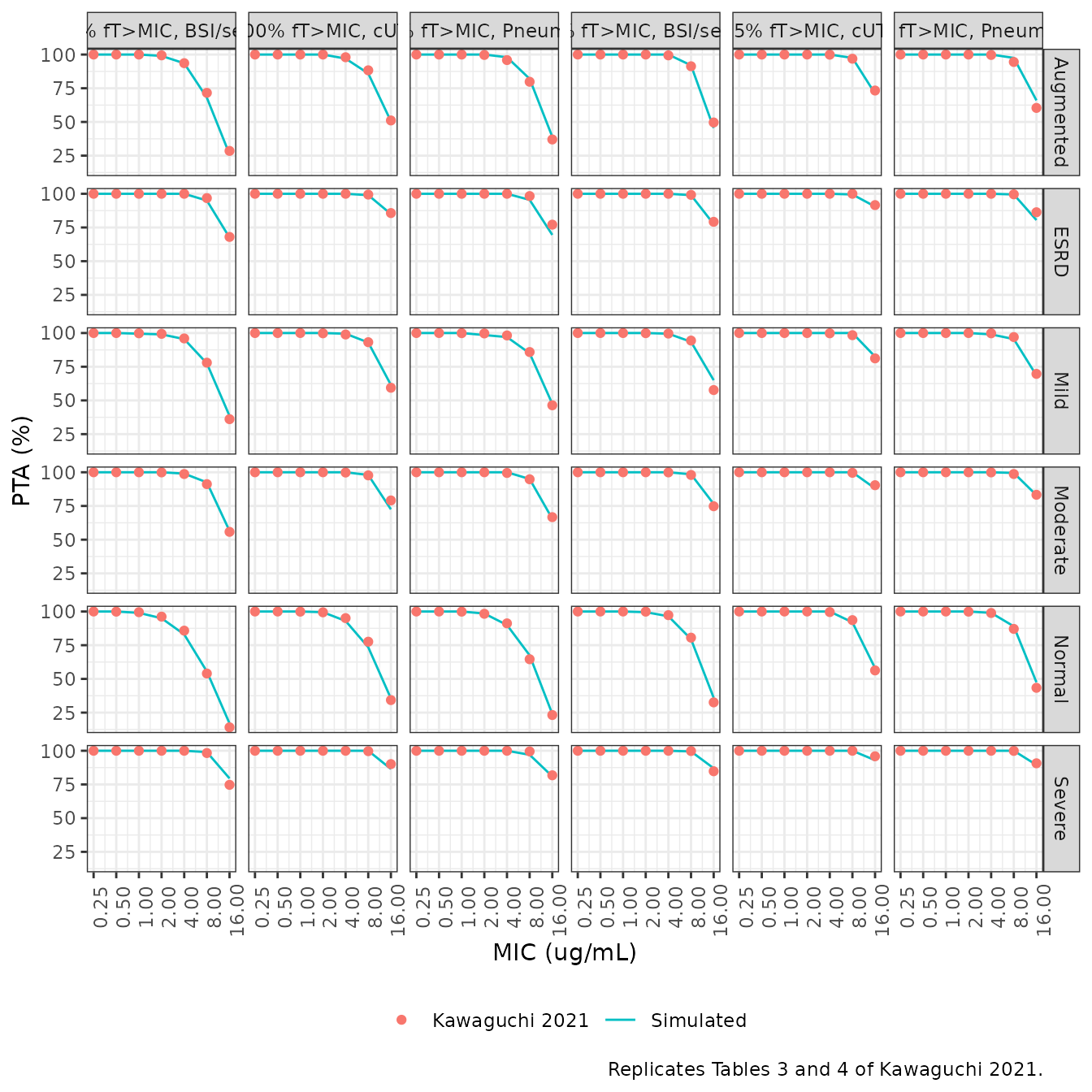
The agreement is measured over every cell, and separately over the cells whose paper value is below 99% (where attainment is not saturated and the comparison actually discriminates). With 200 patients per row the binomial standard error at a 50% PTA is 3.5 percentage points, so a few points of scatter is expected.
disc <- pta_cmp |> filter(paper < 99)
summary_pta <- c(
  n_cells = nrow(pta_cmp),
  n_discriminating = nrow(disc),
  median_diff = median(disc$diff),
  median_abs_diff = median(abs(disc$diff)),
  p90_abs_diff = unname(quantile(abs(disc$diff), 0.9)),
  max_abs_diff_all = max(abs(pta_cmp$diff))
)
round(summary_pta, 2)
#>          n_cells n_discriminating      median_diff  median_abs_diff
#>           252.00            76.00            -0.25             1.40
#>     p90_abs_diff max_abs_diff_all
#>             4.10             7.60
stopifnot(
  nrow(disc) >= 30,
  # Centre: a mis-transcribed clearance or unbound fraction shifts every
  # non-saturated cell in one direction by far more than this.
  abs(median(disc$diff)) < 3,
  median(abs(disc$diff)) < 4,
  quantile(abs(disc$diff), 0.9) < 8
)
Figure 4 – integrated PTA and the text’s breakpoint claims
The integrated PTA weights the renal-function groups by the phase 3 CRCL distribution (Materials and Methods: 20.3%, 15.0%, 24.6%, 32.6%, 4.8% and 2.7% from augmented to ESRD). The Results state that the highest MIC reaching >90% integrated PTA was 8 ug/mL for 75% fT>MIC regardless of infection site, and 4 ug/mL for 100% fT>MIC. Figure 4 itself is not digitised here; instead the same weighting is applied both to the simulation and to the paper’s Tables 3-4.
weights <- data.frame(
  renal = regimens$renal,
  w = c(20.3, 15.0, 24.6, 32.6, 4.8, 2.7) / 100
)
integ <- pta_cmp |>
  inner_join(weights, by = "renal") |>
  group_by(site, target, mic) |>
  summarise(sim = sum(w * sim) / sum(w), paper = sum(w * paper) / sum(w),
            .groups = "drop")
ggplot(integ, aes(mic, sim, colour = site)) +
  geom_line() +
  geom_point(aes(y = paper), shape = 1) +
  geom_hline(yintercept = 90, linetype = 2) +
  facet_wrap(~ paste0(target, "% fT>MIC")) +
  scale_x_log10(breaks = mics, labels = format(mics)) +
  labs(x = "MIC (ug/mL)", y = "Integrated PTA (%)", colour = NULL,
       caption = paste("Lines: simulated. Open circles: the same weighting",
                       "applied to Tables 3-4. Replicates Figure 4.")) +
  theme_bw()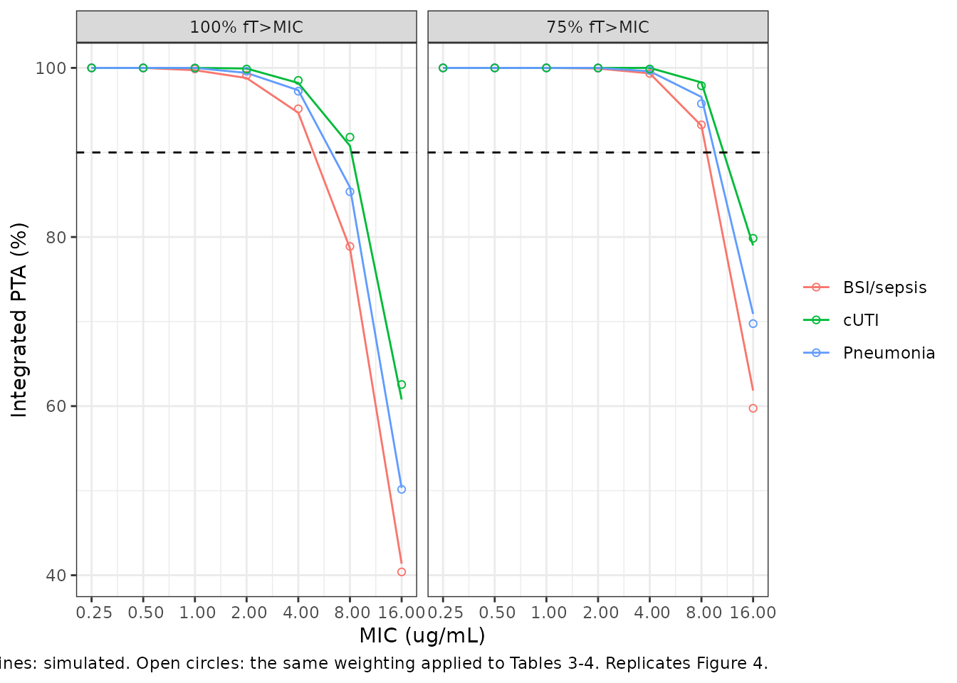
highest_mic <- integ |>
  group_by(site, target) |>
  summarise(
    simulated = max(mic[sim > 90]),
    from_tables = max(mic[paper > 90]),
    sim_at_8 = sim[mic == 8], tables_at_8 = paper[mic == 8],
    .groups = "drop"
  )
knitr::kable(highest_mic, digits = 1, caption = paste(
  "Highest MIC with integrated PTA above 90%, from the simulation and from",
  "the same weighting applied to Tables 3-4, with the integrated PTA at",
  "MIC 8 ug/mL."
))| site | target | simulated | from_tables | sim_at_8 | tables_at_8 |
|---|---|---|---|---|---|
| BSI/sepsis | 75 | 8 | 8 | 93.2 | 93.3 |
| BSI/sepsis | 100 | 4 | 4 | 78.7 | 78.9 |
| Pneumonia | 75 | 8 | 8 | 96.6 | 95.8 |
| Pneumonia | 100 | 4 | 4 | 85.9 | 85.4 |
| cUTI | 75 | 8 | 8 | 98.3 | 97.9 |
| cUTI | 100 | 8 | 8 | 90.8 | 91.8 |
stopifnot(
  nrow(highest_mic) == 6,
  # Integrated PTA tracks the paper's tables at every MIC.
  max(abs(integ$sim - integ$paper)) < 4,
  # 75% fT>MIC: 8 ug/mL for every infection site, as the Results state.
  all(highest_mic$simulated[highest_mic$target == 75] == 8),
  # 100% fT>MIC: 4 ug/mL for pneumonia and BSI/sepsis.
  all(highest_mic$simulated[highest_mic$target == 100 & highest_mic$site != "cUTI"] == 4)
)
For 100% fT>MIC in cUTI the text’s “4 ug/mL” cannot be reproduced
from the paper’s own Table 4: weighting its cUTI rows gives 91.8% at 8
ug/mL, just above the 90% line, and the simulation gives 90.8%. The cUTI
cell sits on the 90% threshold, so its “highest MIC” is not a stable
quantity and is not asserted; its integrated PTA is covered by the
max(abs(sim - paper)) check above.
PKNCA validation
NCA over the steady-state dosing interval for the pneumonia arms (the largest infected population in the analysis).
nca_ids <- cohort |> filter(site == "Pneumonia") |> pull(id)
sim_nca <- sim |>
  filter(id %in% nca_ids, abs(time / 0.25 - round(time / 0.25)) < 1e-8) |>
  select(id, time, Cc, treatment)
dose_df <- cohort |>
  filter(id %in% nca_ids) |>
  transmute(id, time = 0, amt = dose_mg, treatment)

conc_obj <- PKNCA::PKNCAconc(sim_nca, Cc ~ time | treatment + id,
                             concu = "ug/mL", timeu = "h")
dose_obj <- PKNCA::PKNCAdose(dose_df, amt ~ time | treatment + id,
                             doseu = "mg")
intervals <- cohort |>
  filter(id %in% nca_ids) |>
  distinct(treatment, tau) |>
  transmute(treatment, start = 0, end = tau, cmax = TRUE, tmax = TRUE,
            cmin = TRUE, cav = TRUE, auclast = TRUE)
nca_res <- PKNCA::pk.nca(
  PKNCA::PKNCAdata(conc_obj, dose_obj, intervals = intervals)
)
nca_tbl <- as.data.frame(nca_res$result)
stopifnot(nrow(nca_tbl) > 0, !anyNA(nca_tbl$PPORRES))
Steady-state mass balance
At steady state, CL * AUC(0-tau) = Dose for every
subject.
cl_ind <- sim |> filter(id %in% nca_ids) |> distinct(id, cl, dose_mg)
mb <- nca_tbl |>
  filter(PPTESTCD == "auclast") |>
  select(id, auc = PPORRES) |>
  inner_join(cl_ind, by = "id") |>
  mutate(pct = 100 * (cl * auc / dose_mg - 1))
summary(mb$pct)
#>       Min.    1st Qu.     Median       Mean    3rd Qu.       Max.
#> -0.1674356 -0.0211749 -0.0082339 -0.0162710 -0.0029332 -0.0004021
stopifnot(
  nrow(mb) == length(nca_ids),
  abs(median(mb$pct)) < 1,
  quantile(abs(mb$pct), 0.95) < 2
)
Comparison against the published exposure
The Discussion reports geometric-mean daily AUC from the phase 3 post
hoc estimates: 1,365 ug*h/mL at 2 g q6h in patients with
augmented renal function, and 1,494 ug*h/mL at 2 g q8h in
patients with normal renal function. These are empirical summaries of
the enrolled patients (whose covariates are not published), not
typical-value predictions, so the comparison is corroborative. Daily AUC
is 24 * Cavg; the published values are shown as the
equivalent Cavg. The 2 g q8h group is taken as the simulated normal and
mild arms together (CRCL 60 to <120 mL/min, the range that receives 2
g q8h).
simulated <- nca_tbl |>
  filter(PPTESTCD == "cav") |>
  mutate(group = case_when(
    grepl("Augmented", treatment) ~ "2 g q6h, augmented",
    grepl("Normal|Mild", treatment) ~ "2 g q8h, normal",
    TRUE ~ NA_character_
  )) |>
  filter(!is.na(group)) |>
  group_by(group, PPTESTCD) |>
  summarise(PPORRES = exp(mean(log(PPORRES))), .groups = "drop")
published <- data.frame(
  group = c("2 g q6h, augmented", "2 g q8h, normal"),
  cav = c(1365, 1494) / 24
)
cmp <- nlmixr2lib::ncaComparisonTable(
  simulated = simulated,
  reference = published,
  by = "group",
  units = c(cav = "ug/mL"),
  tolerance_pct = 20
)
knitr::kable(cmp, caption = paste(
  "Simulated geometric-mean steady-state Cavg (pneumonia patients) against",
  "the Discussion's phase 3 geometric-mean daily AUC divided by 24 h.",
  "* differs from reference by more than 20%."
))| NCA parameter | group | Reference | Simulated | % diff |
|---|---|---|---|---|
| Cavg (ug/mL) | 2 g q6h, augmented | 56.9 | 60.4 | +6.2% |
| Cavg (ug/mL) | 2 g q8h, normal | 62.2 | 60.9 | -2.2% |
Assumptions and deviations
-
Covariate encoding. The paper’s infection-site
variable (
PTin Table S2) is split into mutually exclusive indicatorsDIS_PNEUMONIA,DIS_BACTEREMIA(the paper’s BSI/sepsis category) andDIS_CUTI(cUTI, pooled with acute uncomplicated pyelonephritis in the phase 2 study). The any-infection factor on V1 is applied to their sum. The pneumonia arm pooled hospital-acquired, ventilator-associated and health care-associated pneumonia under one coefficient, so the general pneumonia flag is used. -
Study-specific cUTI effect. The cUTI factor on CL
differs between the phase 2 APEKS-cUTI study (1.27) and the phase 3
CREDIBLE-CR study (0.872); the control stream switches on the subject
ID. The packaged model uses a
STUDY_CEFIDEROCOL_PHASE2indicator, whose default of 0 gives the CREDIBLE-CR value that the paper used in its own simulations. - Albumin units. The model was calibrated in g/dL (reference 3.9 g/dL). The packaged model takes albumin in g/L and divides by 10 internally.
- Albumin exponent sign. The article’s typeset minus sign (-0.617) is confirmed by the control stream’s bounds for THETA(14), (-2.0, -0.5, 0.5), and by the Discussion (lower albumin, larger V1).
- Time-varying creatinine clearance. The source data used baseline CRCL for the phase 1 and phase 2 studies and time-varying CRCL for the phase 3 studies; the packaged model accepts either.
- Virtual cohort details not stated in the paper. The log-normal body weight and albumin distributions are parameterised with the stated means as arithmetic means. The upper bound for the augmented group above 150 mL/min is set at 200 mL/min, which has no effect on CL because of the 150 mL/min cap. CRCL is uniform within each group. The paper’s %fT>MIC is taken without residual error; simulating 200 rather than 1,000 patients per scenario adds a few points of binomial scatter to each PTA cell.
- Integrated PTA claim for cUTI. The Results state that the highest MIC with more than 90% integrated PTA for 100% fT>MIC was 4 ug/mL. Applying the stated renal-function weights to the paper’s own Table 4 gives 91.8% for cUTI at 8 ug/mL, so for cUTI the statement holds only if Figure 4 was computed slightly differently from the tables. Pneumonia and BSI/sepsis agree with the statement, and the simulated cUTI value (about 91%) sits on the same threshold as the tables.