Bispecific antibody minimal PBPK-PD: BITS7201A, mosunetuzumab and a tumor-targeted bispecific (Spinosa 2026)
Source:vignettes/articles/Spinosa_2026_bispecific_mpbpk.Rmd
Spinosa_2026_bispecific_mpbpk.RmdModel and source
- Citation: Spinosa P, Joslyn L, Ramanujan S, Gadkar K, Hosseini I. A Generalized Minimal PBPK-PD Model of Bispecific Antibodies: Case Studies and Applications in Drug Development. CPT Pharmacometrics Syst Pharmacol. 2026;15(2):e70167.
- Article: https://doi.org/10.1002/psp4.70167 (open access, PMC12896375)
- Supplement: Data S1, a zip holding the model description
(
-s01.docx), Tables S1-S4 (-s02.docx), the SimBiology project (-s04.sbproj), two MATLAB helper functions (-s05.m,-s06.m) and the parameter workbook (-s07.xlsx, one sheet per case study).
Spinosa et al. built one generalized minimal PBPK model for bispecific antibodies. It extends the second-generation Cao-Jusko minimal PBPK backbone (plasma, leaky and tight interstitial tissue, lymph; Cao 2013) with optional safety and efficacy tissues, two targets that may each be soluble or membrane-bound in every compartment except lymph, and three binding modes: both arms on soluble targets, trans-binding of two receptors on different cells (T-cell engagers), and cis-binding of two receptors on the same cell (tumor-targeted bispecifics), with a bivalent monospecific antibody as a further option. Flags in the SimBiology project switch the modes on and off, and the workbook supplies one parameter set per case study.
The library ships the four molecules the paper actually parameterizes. Each file is the published model reduced to the species that can become non-zero under that case study’s flags and target burden, so every equation is the published rate law with the switched-off terms dropped:
| Model | Case study | Binding mode | Species |
|---|---|---|---|
Spinosa_2026_BITS7201A_mpbpk |
1, anti-IL-13/IL-17AA | two soluble targets, complexes traffic | human |
Spinosa_2026_mosunetuzumab_cyno_mpbpk |
2 (and 3), CD20 x CD3 | trans-binding, central targets | cynomolgus monkey |
Spinosa_2026_tumor_targeted_bsab_mpbpk |
4, prototypical tumor-targeted bispecific | cis-binding with avidity | human |
Spinosa_2026_bivalent_mab_mpbpk |
4, bivalent comparator | bivalent with avidity | human |
The reductions were checked against a direct translation of the complete published model (all 81 differential equations and 273 reactions of the SimBiology project, with the workbook parameters): the two encodings agree to better than one part in 10^7 for every state compared.
mod_bits <- readModelDb("Spinosa_2026_BITS7201A_mpbpk")
mod_mosun <- readModelDb("Spinosa_2026_mosunetuzumab_cyno_mpbpk")
mod_tt <- readModelDb("Spinosa_2026_tumor_targeted_bsab_mpbpk")
mod_bv <- readModelDb("Spinosa_2026_bivalent_mab_mpbpk")

rx_bits <- rxode2::rxode2(mod_bits)
rx_mosun <- rxode2::rxode2(mod_mosun)
rx_tt <- rxode2::rxode2(mod_tt)
rx_bv <- rxode2::rxode2(mod_bv)

# The models carry no inter-individual variability, so every multi-subject
# solve below differs only in its doses or parameter columns; rxode2's
# "multi-subject simulation without 'omega'" note is expected and muffled.
solve_typical <- function(...) {
  withCallingHandlers(
    rxode2::rxSolve(...),
    warning = function(w) {
      if (grepl("without 'omega'", conditionMessage(w), fixed = TRUE)) invokeRestart("muffleWarning")
    }
  )
}
Population
The model is mechanistic and calibrated to mean-level data, so none of the four files carries inter-individual variability or a residual-error estimate.
- Case Study 1 (BITS7201A). Healthy volunteers in the phase I single- and multiple-ascending-dose study of Staton et al. (BMC Pulm Med 2019). The model was calibrated to the SAD cohorts (30, 90 and 300 mg SC; 300 and 750 mg IV) and validated against the MAD cohorts (150, 300 and 600 mg SC every 4 weeks x 3). A 70 kg body weight scales the per-kg volumes for flat-mg doses.
- Case Studies 2 and 3 (mosunetuzumab). Cynomolgus monkeys given 0.01, 0.1 or 1 mg/kg IV once weekly for 4 weeks (Hosseini et al., NPJ Syst Biol Appl 2020). Only the nonspecific clearance was fitted to mosunetuzumab PK; the CD3 and CD20 capacities were fitted beforehand to other molecules (Figure 4).
- Case Study 4 (tumor-targeted bispecific and bivalent comparator). A simulation-only design study in a 70 kg patient with a solid tumor.
Source trace
Every model shares the minimal PBPK transport: free drug leaves
plasma for each tissue i at
L_i (1 - sigma_i) C_plasma / V_plasma (in plasma units),
leaves the tissue for lymph at L_i (1 - sigma_L) C_i / V_i,
and returns from lymph at L C_lymph / V_lymph, with
L_i = f_i L. The receiving compartment gains the same
amount, so each flux is multiplied by the volume ratio (Data S1,
transport_between_compartments in -s05.m).
Binding is kon (D R - KD C) for a first binding and
chi kon C1 R2 - kon KD C12 for the second (Data S1,
binding_on_off in -s06.m). Receptors are
synthesized at kdeg R0 and degraded at kdeg;
receptor-bound drug is internalized at kdeg (the workbook’s
fold change fcint is 1).
| Quantity | Value | Source |
|---|---|---|
| Shared physiology | ||
Lymph flow L
|
41.4288 mL/day/kg | Workbook L_D1 (all sheets) |
| Leaky / tight volumes | 62.4 / 115.9 mL/kg | Workbook V_lea, V_tig
|
| Tight reflection coefficient | 0.95 | Workbook sig_tig_D1
|
| Lymphatic reflection coefficient | 0.2 | Workbook sig_lym_D1
|
| Antibody molecular weight | 150 000 g/mol | Workbook MWab_D1; Data S1 “150 kDa” |
| kon (every arm) | 3.6 1/nM/day | Workbook kon_R1_D1, kon_R2_D1
|
| BITS7201A | ||
| CLns | 3.1 mL/kg/day | Table S1; workbook CLp_D1
|
| Vplasma | 52 mL/kg | Table S1 (inferred from Cmax); workbook V_cen
|
| Vlymph | 37.14 mL/kg | Workbook V_lym
|
| kabs, F | 0.2 1/day, 0.92 | Table S1; workbook kabs_D1, F_D1
|
| Leaky reflection, lymph-flow split | 0.7; 0.65 / 0.35 | Workbook sig_lea_D1, f_lea_D1,
f_tig_D1
|
| KD IL-13 / IL-17AA | 0.005 / 0.010 nM | Table S1; workbook Kd_R1_D1, Kd_R2_D1
|
| Baseline IL-13 / IL-17AA | 6e-6 / 2.83e-6 nM | Workbook sR1_0_*, sR2_0_* (Table S1 ranges
in pg/mL) |
| Turnover half-life IL-13 / IL-17AA | 0.0208 / 0.0056 day | Workbook Thalf_sR1, Thalf_sR2 (Table S1:
30 / 8 min) |
| Body weight | 70 kg | Workbook BW
|
| Mosunetuzumab (cyno) | ||
| CLns | 4.0 mL/kg/day | Table S2 (fitted); workbook CLp_D1
|
| Vplasma / Vlymph | 37.14 / 44.4 mL/kg | Workbook V_cen, V_lym
|
| Leaky reflection, lymph-flow split | 0.67; 0.65 / 0.35 | Workbook sig_lea_D1, f_lea_D1,
f_tig_D1
|
| KD CD20 / CD3 | 68 / 40 nM | Table S2; workbook Kd_R1_D1, Kd_R2_D1
|
| CD20 / CD3 capacity | 4.4 / 19 nM | Table S2 (fit; +/-30% ranges) |
| CD20 / CD3 turnover half-life | 1.0 / 0.7083 day | Table S2 (1.0 / 0.7 day); workbook Thalf_mR1,
Thalf_mR2
|
| Trans-binding avidity | 1 | Data S1 text (“avidity constant is equal to 1”) |
| Tumor-targeted bispecific / bivalent comparator | ||
| CLns | 2.8272 mL/kg/day | Workbook CLp_D1; Table S4 (2.8) |
| Vplasma / Vtumor / Vlymph | 37.14 / 4 / 37.14 mL/kg | Workbook V_cen, V_eff,
V_lym
|
| Lymph-flow split leaky / tight / tumor | 0.58 / 0.35 / 0.07 | Workbook f_lea_D1, f_tig_D1,
f_eff_D1
|
| Leaky and tumor reflection | 0.7 | Workbook sig_lea_D1, sig_eff_D1
|
| KD therapeutic / targeting (bispecific) | 100 / 0.05 nM | Table S4; workbook Kd_R1_D1, Kd_R2_D1
|
| KD therapeutic (bivalent) | 10 nM | Table S4 |
| Cells, receptors per cell | 10^6 /mL; 10^4 therapeutic everywhere, 10^3 targeting (10^5 in tumor) | Table S3; workbook mR*_cellspermL_*,
rpc_mR*_*
|
| Receptor turnover half-life | 1 day | Workbook Thalf_mR1, Thalf_mR2
|
| Effective avidity, therapeutic arm second | 1000 | Figure 7 caption; workbook avid_R1_D1 = 1e9 per 10^6
cells/mL |
| Effective avidity, targeting arm second | 1e-6 | Workbook avid_R2_D1 = 1 per 10^6 cells/mL |
| Effective avidity, bivalent second arm | 1000 | Project variant “6. AVIDITY: same cell bv mAb” (1e9 per 10^6 cells/mL) |
Case Study 1: BITS7201A (anti-IL-13 / anti-IL-17AA)
Single ascending dose PK (Figure 2b,c)
sad <- tibble::tribble(
  ~treatment, ~amt, ~cmt,
  "30 mg SC", 30, "depot",
  "90 mg SC", 90, "depot",
  "300 mg SC", 300, "depot",
  "300 mg IV", 300, "central",
  "750 mg IV", 750, "central"
) |>
  mutate(id = row_number())
obs_times <- sort(unique(c(0, seq(0.25, 3, by = 0.25), seq(3.5, 84, by = 0.5))))
ev_sad <- bind_rows(
  sad |> mutate(time = 0, evid = 1),
  tidyr::crossing(sad |> select(id, treatment, cmt), time = obs_times) |>
    mutate(amt = 0, evid = 0)
) |>
  arrange(id, time, desc(evid)) |>
  select(id, time, amt, evid, cmt, treatment)

sim_sad <- solve_typical(rx_bits, ev_sad, keep = "treatment", returnType = "data.frame")
sim_sad$treatment <- factor(sim_sad$treatment, levels = sad$treatment)

ggplot(sim_sad, aes(time, Cc, colour = treatment)) +
  geom_line() +
  scale_y_log10(limits = c(0.01, 1000)) +
  labs(x = "Time (days)", y = "Total BITS7201A (ug/mL)", colour = NULL,
       caption = "Replicates Figure 2b,c of Spinosa 2026 (model lines only).")
#> Warning in scale_y_log10(limits = c(0.01, 1000)): log-10 transformation
#> introduced infinite values.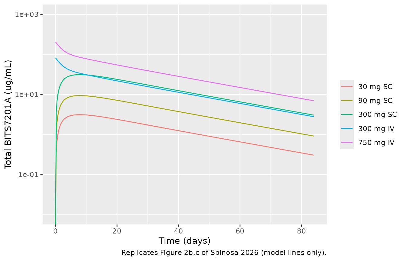
Multiple ascending dose PK and serum IL-17AA (Figure 3a,b)
The MAD cohorts received three SC doses every 4 weeks. Total serum IL-17AA (free plus drug-bound) rises because the drug-bound cytokine is cleared at the antibody’s slow clearance instead of the cytokine’s minutes-long turnover. The paper captures the spread of the data by varying the unmeasurable baseline IL-17AA between 0.04 and 0.3 pg/mL; the model works in nM and the paper reports no molecular weight for IL-17AA, so the band below brackets the nominal baseline with the low (1e-6 nM) and high (8.753e-6 nM) baselines stored as variants in the published SimBiology project.
mad <- tibble::tibble(treatment = c("150 mg SC q4w", "300 mg SC q4w", "600 mg SC q4w"),
                      dose = c(150, 300, 600))
mad_times <- seq(0, 140, by = 1)
mad_ev <- function(bl) {
  bind_rows(
    tidyr::crossing(mad, time = c(0, 28, 56)) |> mutate(amt = dose, evid = 1, cmt = "depot"),
    tidyr::crossing(mad, time = mad_times) |> mutate(amt = 0, evid = 0, cmt = "central")
  ) |>
    mutate(id = as.integer(factor(treatment, levels = mad$treatment)), bl_il17 = bl) |>
    arrange(id, time, desc(evid))
}
sim_mad <- bind_rows(lapply(c(low = 1e-6, nominal = 2.83e-6, high = 8.753e-6), function(bl) {
  solve_typical(rx_bits, mad_ev(bl), keep = "treatment", returnType = "data.frame")
}), .id = "baseline")

ggplot(sim_mad |> filter(baseline == "nominal"), aes(time, Cc, colour = treatment)) +
  geom_line() +
  scale_y_log10(limits = c(0.01, 1000)) +
  scale_x_continuous(breaks = seq(0, 140, 28)) +
  labs(x = "Time (days)", y = "Total BITS7201A (ug/mL)", colour = NULL,
       caption = "Replicates Figure 3a of Spinosa 2026.")
#> Warning in scale_y_log10(limits = c(0.01, 1000)): log-10 transformation
#> introduced infinite values.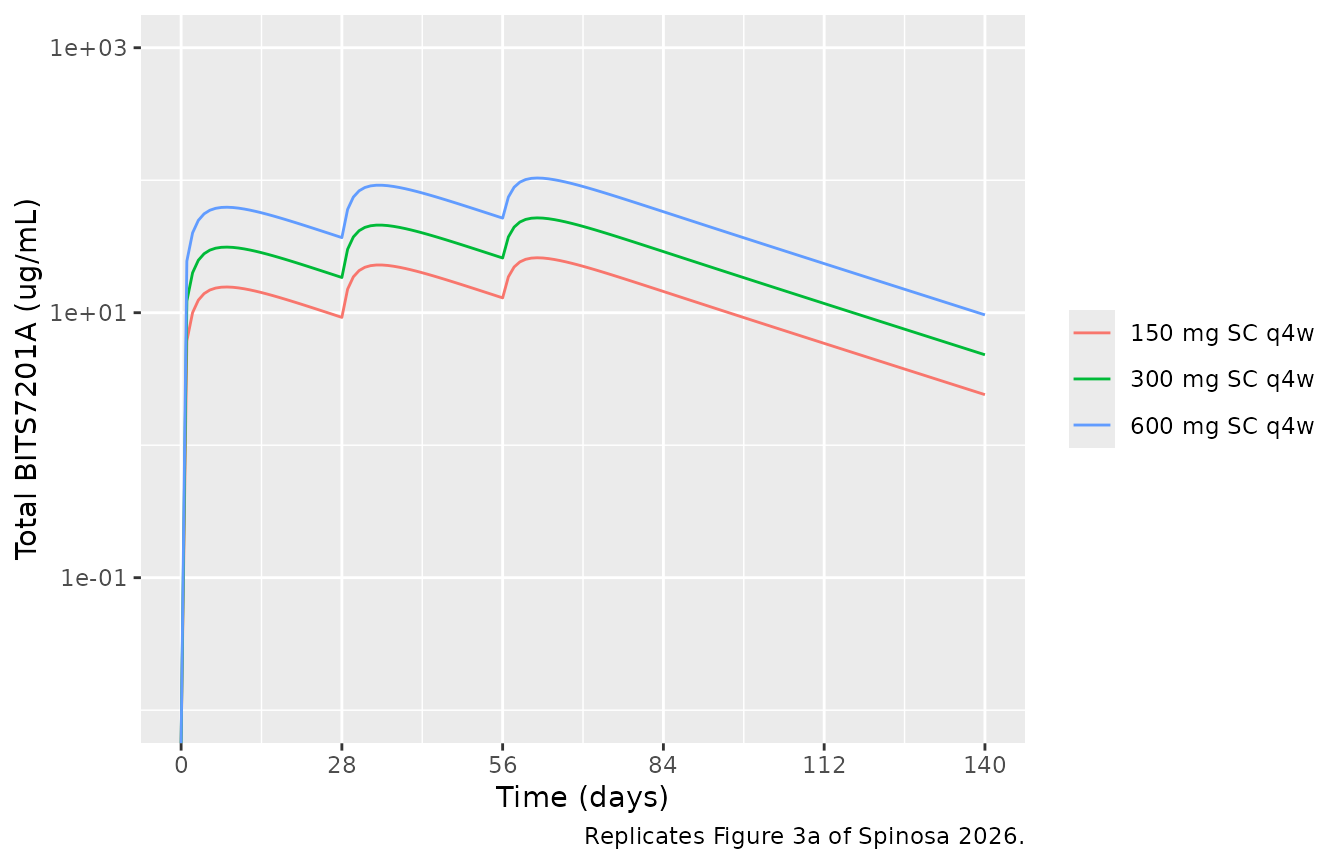
sim_mad |>
  select(baseline, treatment, time, il17_total_central) |>
  tidyr::pivot_wider(names_from = baseline, values_from = il17_total_central) |>
  ggplot(aes(time, nominal * 1e6)) +
  geom_ribbon(aes(ymin = low * 1e6, ymax = high * 1e6), alpha = 0.3) +
  geom_line() +
  facet_wrap(~treatment) +
  scale_x_continuous(breaks = seq(0, 140, 28)) +
  labs(x = "Time (days)", y = "Total serum IL-17AA (fM)",
       caption = "Replicates Figure 3b of Spinosa 2026 in molar units; band = baseline range.")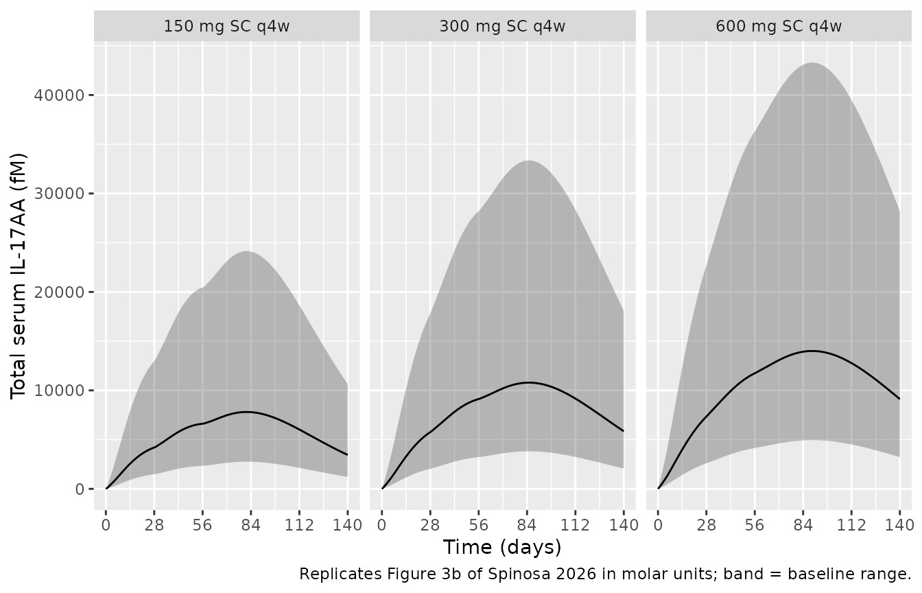
Target neutralization in serum and tissue (Figure 3d,e)
Figure 3d,e plots free target as a percentage of baseline at day 28 after a single IV dose. The paper states that the highest SAD dose (750 mg) neutralizes about 80% of serum IL-17AA and about 90% of serum IL-13, and the figure shows the tight tissue, which drug reaches slowly, staying least neutralized.
iv_doses <- c(10, 30, 100, 300, 750, 1000, 3000, 10000)
ev_iv <- tibble::tibble(id = seq_along(iv_doses), dose = iv_doses) |>
  tidyr::crossing(time = c(0, 28)) |>
  mutate(amt = ifelse(time == 0, dose, 0), evid = ifelse(time == 0, 1, 0), cmt = "central")
neut <- solve_typical(rx_bits, ev_iv, keep = "dose", returnType = "data.frame") |>
  filter(time == 28) |>
  select(dose, starts_with("il17_pctfree"), starts_with("il13_pctfree")) |>
  tidyr::pivot_longer(-dose, names_to = c("cytokine", "location"),
                      names_pattern = "(il1[37])_pctfree_(.*)", values_to = "pct_free")

ggplot(neut, aes(dose, pct_free, linetype = location)) +
  geom_line() +
  facet_wrap(~cytokine, labeller = as_labeller(c(il13 = "IL-13", il17 = "IL-17AA"))) +
  scale_x_log10() +
  labs(x = "IV dose (mg)", y = "Free target at day 28 (% of baseline)", linetype = NULL,
       caption = "Replicates Figure 3d,e of Spinosa 2026.")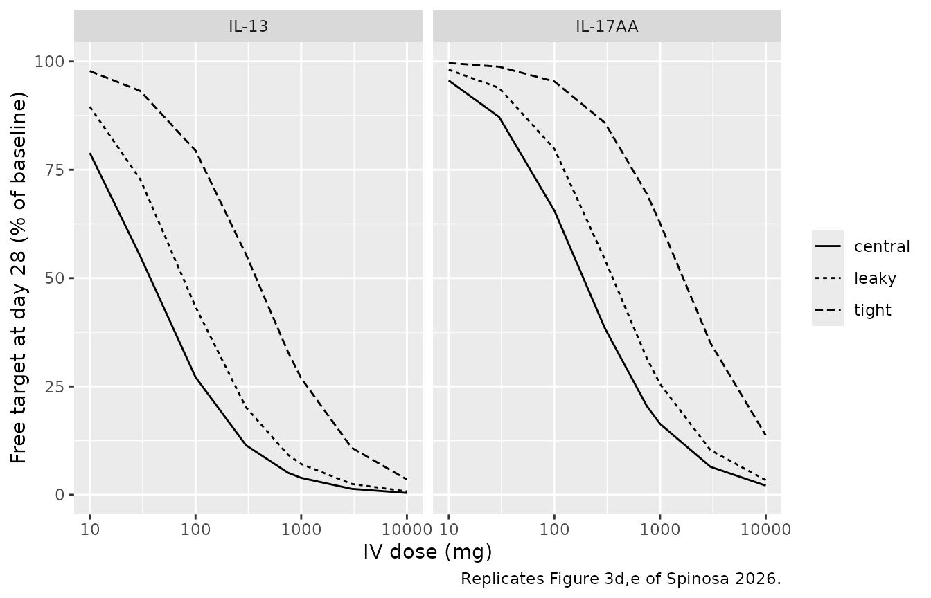
neut_750 <- neut |> filter(dose == 750)
knitr::kable(neut_750 |> mutate(pct_free = round(pct_free, 1)) |>
  dplyr::rename("IV dose (mg)" = dose, "Cytokine" = cytokine, "Compartment" = location,
                "Free target, % of baseline" = pct_free),
caption = "Day-28 free cytokine after 750 mg IV.")| IV dose (mg) | Cytokine | Compartment | Free target, % of baseline |
|---|---|---|---|
| 750 | il17 | central | 20.5 |
| 750 | il17 | leaky | 31.5 |
| 750 | il17 | tight | 69.4 |
| 750 | il13 | central | 5.1 |
| 750 | il13 | leaky | 9.2 |
| 750 | il13 | tight | 32.9 |
pf <- function(cyt, loc, d) {
  vapply(d, function(dd) neut$pct_free[neut$cytokine == cyt & neut$location == loc & neut$dose == dd], numeric(1))
}
stopifnot(
  # Paper text: 750 mg neutralizes ~80% of IL-17AA and ~90% of IL-13 in serum.
  abs(pf("il17", "central", 750) - 20) < 5,
  pf("il13", "central", 750) < 10,
  # Figure 3d,e ordering at every dose: central < leaky < tight free target.
  all(pf("il17", "central", iv_doses) < pf("il17", "leaky", iv_doses)),
  all(pf("il17", "leaky", iv_doses) < pf("il17", "tight", iv_doses)),
  # Figure 3d at 1000 mg reads ~17 / ~25 / ~65% free IL-17AA.
  abs(pf("il17", "tight", 1000) - 65) < 10
)
PKNCA of the SAD cohorts
The paper does not tabulate NCA results, so there is no published reference to compare against; the NCA below documents the simulated typical-subject exposure and confirms the linear (dose-proportional) PK the paper describes for the SAD range.
sim_nca <- sim_sad |>
  dplyr::filter(!is.na(Cc)) |>
  dplyr::select(id, time, Cc, treatment)
sim_nca <- dplyr::bind_rows(
  sim_nca,
  sim_nca |> dplyr::distinct(id, treatment) |> dplyr::mutate(time = 0, Cc = 0)
) |>
  dplyr::distinct(id, treatment, time, .keep_all = TRUE) |>
  dplyr::arrange(id, treatment, time)
conc_obj <- PKNCA::PKNCAconc(sim_nca, Cc ~ time | treatment + id)
dose_df <- ev_sad |> dplyr::filter(evid == 1) |> dplyr::select(id, time, amt, treatment)
dose_obj <- PKNCA::PKNCAdose(dose_df, amt ~ time | treatment + id)
intervals <- data.frame(start = 0, end = 84, cmax = TRUE, tmax = TRUE, auclast = TRUE)
nca_res <- PKNCA::pk.nca(PKNCA::PKNCAdata(conc_obj, dose_obj, intervals = intervals))
nca_tab <- as.data.frame(nca_res) |>
  select(treatment, PPTESTCD, PPORRES) |>
  tidyr::pivot_wider(names_from = PPTESTCD, values_from = PPORRES) |>
  left_join(sad |> select(treatment, amt), by = "treatment")
knitr::kable(nca_tab |> mutate(across(c(cmax, auclast), \(x) signif(x, 3))) |>
  dplyr::rename("Group" = treatment, "Cmax (ug/mL)" = cmax, "Tmax (day)" = tmax,
                "AUC0-84 (ug*day/mL)" = auclast, "Dose (mg)" = amt),
caption = "Simulated NCA of total BITS7201A, SAD cohorts.")| Group | AUC0-84 (ug*day/mL) | Cmax (ug/mL) | Tmax (day) | Dose (mg) |
|---|---|---|---|---|
| 30 mg SC | 118 | 3.13 | 8 | 30 |
| 300 mg IV | 1290 | 82.40 | 0 | 300 |
| 300 mg SC | 1180 | 31.30 | 8 | 300 |
| 750 mg IV | 3240 | 206.00 | 0 | 750 |
| 90 mg SC | 353 | 9.38 | 8 | 90 |
Case Study 2: mosunetuzumab in cynomolgus monkeys
Multi-dose PK with the CD3 / CD20 capacity range (Figure 5d)
The shaded band is the paper’s +/-30% range on both receptor capacities (CD3 13-25 nM, CD20 3.3-5.8 nM).
mosun_doses <- c(0.01, 0.1, 1)
mosun_times <- sort(unique(c(seq(0, 40, by = 0.25), 6.999, 13.999, 20.999)))
ev_mosun <- function(scale) {
  bind_rows(
    tidyr::crossing(dose = mosun_doses, time = c(0, 7, 14, 21)) |> mutate(amt = dose, evid = 1),
    tidyr::crossing(dose = mosun_doses, time = mosun_times) |> mutate(amt = 0, evid = 0)
  ) |>
    mutate(id = as.integer(factor(dose)), cmt = "central",
           bl_cd3 = 19 * scale, bl_cd20 = 4.4 * scale,
           treatment = paste(dose, "mg/kg QW")) |>
    arrange(id, time, desc(evid))
}
sim_mosun <- bind_rows(lapply(c(lower = 1.3, nominal = 1, upper = 0.7), function(s) {
  solve_typical(rx_mosun, ev_mosun(s), keep = c("treatment", "dose"), returnType = "data.frame")
}), .id = "capacity")
mosun_wide <- sim_mosun |>
  select(capacity, treatment, dose, time, Cc) |>
  tidyr::pivot_wider(names_from = capacity, values_from = Cc)

ggplot(mosun_wide, aes(time, nominal, colour = treatment, fill = treatment)) +
  geom_ribbon(aes(ymin = lower, ymax = upper), alpha = 0.3, colour = NA) +
  geom_line() +
  scale_y_log10(limits = c(1e-3, 1e4)) +
  labs(x = "Time (days)", y = "Free mosunetuzumab (ug/mL)", colour = NULL, fill = NULL,
       caption = "Replicates Figure 5d of Spinosa 2026 (model lines only).")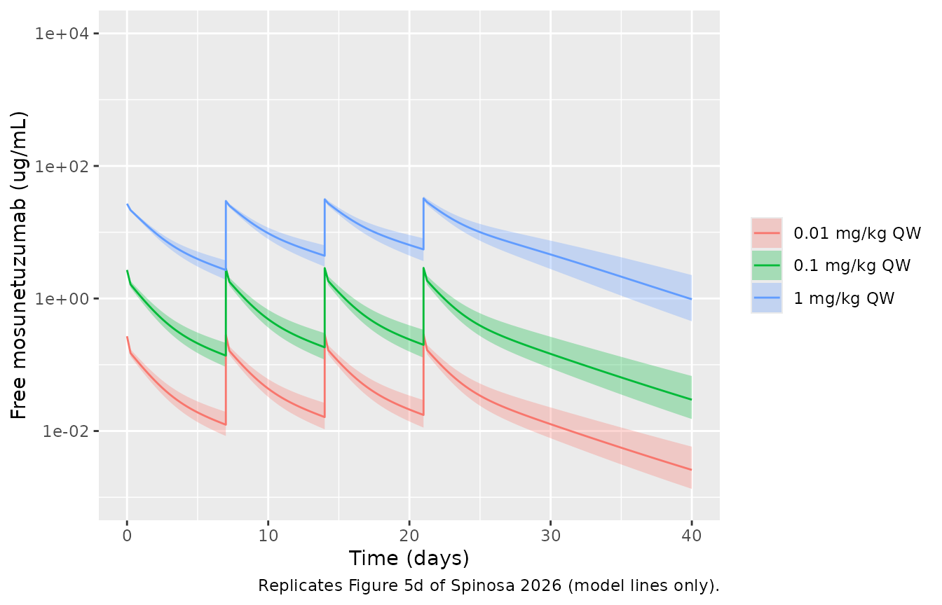
The central line of Figure 5d at day 40 reads roughly 1, 0.03 and 0.0025 ug/mL for 1, 0.1 and 0.01 mg/kg (read off the figure by the maintainers; log axis, so only to within about a factor of 1.5).
day40 <- mosun_wide |> filter(time == 40) |> arrange(dose)
day40$digitized <- c(0.0025, 0.03, 1)
knitr::kable(day40 |> transmute(treatment, simulated = signif(nominal, 3), digitized) |>
  dplyr::rename("Regimen" = treatment, "Simulated day-40 Cc (ug/mL)" = simulated,
"Figure 5d central line (ug/mL)" = digitized))| Regimen | Simulated day-40 Cc (ug/mL) | Figure 5d central line (ug/mL) |
|---|---|---|
| 0.01 mg/kg QW | 0.00259 | 0.0025 |
| 0.1 mg/kg QW | 0.02970 | 0.0300 |
| 1 mg/kg QW | 0.97400 | 1.0000 |
Contribution of T- and B-cell-mediated disposition (Figure 5e,f)
Removing CD3 (no T cells) raises exposure substantially at every dose; removing CD20 (no B cells) has a smaller effect.
sim_noT <- solve_typical(rx_mosun, ev_mosun(1) |> mutate(bl_cd3 = 0),
                           keep = c("treatment", "dose"), returnType = "data.frame")
sim_noB <- solve_typical(rx_mosun, ev_mosun(1) |> mutate(bl_cd20 = 0),
                           keep = c("treatment", "dose"), returnType = "data.frame")
cmp_tmdd <- bind_rows(
  `with T and B cells` = sim_mosun |> filter(capacity == "nominal"),
  `without T cells` = sim_noT,
  `without B cells` = sim_noB,
  .id = "scenario"
)
ggplot(cmp_tmdd, aes(time, Cc, colour = treatment, linetype = scenario)) +
  geom_line() +
  scale_y_log10(limits = c(1e-3, 1e4)) +
  labs(x = "Time (days)", y = "Free mosunetuzumab (ug/mL)", colour = NULL, linetype = NULL,
       caption = "Replicates Figure 5e,f of Spinosa 2026.")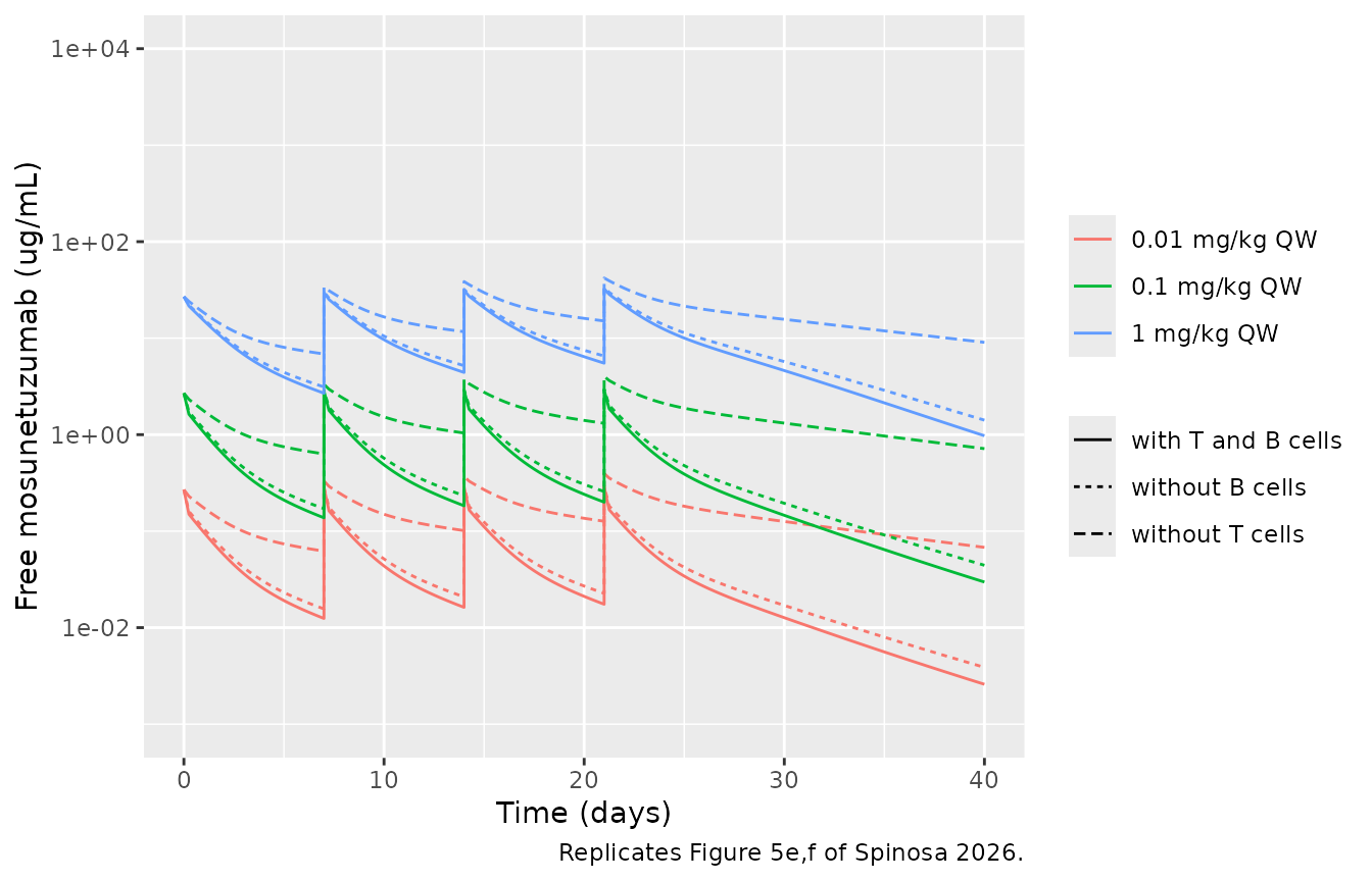
ratio_at <- function(sim, d) {
  sim$Cc[sim$dose == d & sim$time == 40] /
    sim_mosun$Cc[sim_mosun$capacity == "nominal" & sim_mosun$dose == d & sim_mosun$time == 40]
}
stopifnot(
  # T-cell-mediated disposition matters even at the highest dose (Figure 5e).
  ratio_at(sim_noT, 1) > 3,
  # B-cell-mediated disposition matters less than T-cell-mediated (Figure 5f).
  all(sapply(mosun_doses, ratio_at, sim = sim_noB) < sapply(mosun_doses, ratio_at, sim = sim_noT))
)
PKNCA of the first dosing interval
nca_in <- sim_mosun |>
  filter(capacity == "nominal", time <= 6.999, !is.na(Cc)) |>
  select(id, time, Cc, treatment)
# IV bolus into a concentration state: the time-0 record is the post-dose
# concentration, which the solve already returns; assert it is there.
stopifnot(all(tapply(nca_in$time == 0, nca_in$id, any)))
conc2 <- PKNCA::PKNCAconc(nca_in, Cc ~ time | treatment + id)
dose2 <- ev_mosun(1) |> filter(evid == 1, time == 0) |> select(id, time, amt, treatment)
dose2_obj <- PKNCA::PKNCAdose(dose2, amt ~ time | treatment + id, route = "intravascular")
res2 <- PKNCA::pk.nca(PKNCA::PKNCAdata(conc2, dose2_obj,
  intervals = data.frame(start = 0, end = 6.999, cmax = TRUE, auclast = TRUE)))
nca2 <- as.data.frame(res2) |>
  select(treatment, PPTESTCD, PPORRES) |>
  tidyr::pivot_wider(names_from = PPTESTCD, values_from = PPORRES) |>
  mutate(dose = as.numeric(sub(" mg/kg QW", "", treatment)), auc_per_dose = auclast / dose)
knitr::kable(nca2 |> mutate(across(c(cmax, auclast, auc_per_dose), \(x) signif(x, 3))) |>
  dplyr::rename("Regimen" = treatment, "Cmax (ug/mL)" = cmax, "AUC0-7 (ug*day/mL)" = auclast,
                "Dose (mg/kg)" = dose, "AUC0-7 / dose" = auc_per_dose),
caption = "Simulated first-interval NCA of free mosunetuzumab.")| Regimen | AUC0-7 (ug*day/mL) | Cmax (ug/mL) | Dose (mg/kg) | AUC0-7 / dose |
|---|---|---|---|---|
| 0.01 mg/kg QW | 0.345 | 0.269 | 0.01 | 34.5 |
| 0.1 mg/kg QW | 3.730 | 2.690 | 0.10 | 37.3 |
| 1 mg/kg QW | 56.800 | 26.900 | 1.00 | 56.8 |
Case Study 3: CD3 affinity and the share of clearance (Figure 6)
Case Study 3 reuses the mosunetuzumab model setup (workbook sheet “Case Study 3”: the Table S2 capacities, here 19.1 nM CD3 and 4.48 nM CD20 from the receptors-per-mL inputs) and compares a moderate (40 nM) with a low (400 nM) CD3 affinity, plus no CD3 binding, after a single IV dose. The cumulative-elimination states split total clearance by route at day 21.
cs3 <- tidyr::crossing(dose = c(0.01, 0.1, 1, 10),
                       affinity = c("40 nM", "400 nM", "no CD3 binding")) |>
  mutate(id = row_number(),
         kd_cd3 = ifelse(affinity == "400 nM", 400, 40),
         kon_cd3 = ifelse(affinity == "no CD3 binding", 0, 3.6),
         bl_cd3 = 19.097, bl_cd20 = 4.4836)
ev_cs3 <- bind_rows(
  cs3 |> mutate(time = 0, amt = dose, evid = 1),
  tidyr::crossing(cs3, time = seq(0, 21, by = 0.25)) |> mutate(amt = 0, evid = 0)
) |>
  mutate(cmt = "central") |>
  arrange(id, time, desc(evid))
sim_cs3 <- solve_typical(rx_mosun, ev_cs3, keep = c("dose", "affinity"), returnType = "data.frame")

ggplot(sim_cs3, aes(time, Cc, colour = factor(dose), linetype = affinity)) +
  geom_line() +
  scale_y_log10() +
  labs(x = "Time (days)", y = "Free drug (ug/mL)", colour = "Dose (mg/kg)", linetype = "CD3 KD",
       caption = "Replicates Figure 6a of Spinosa 2026.")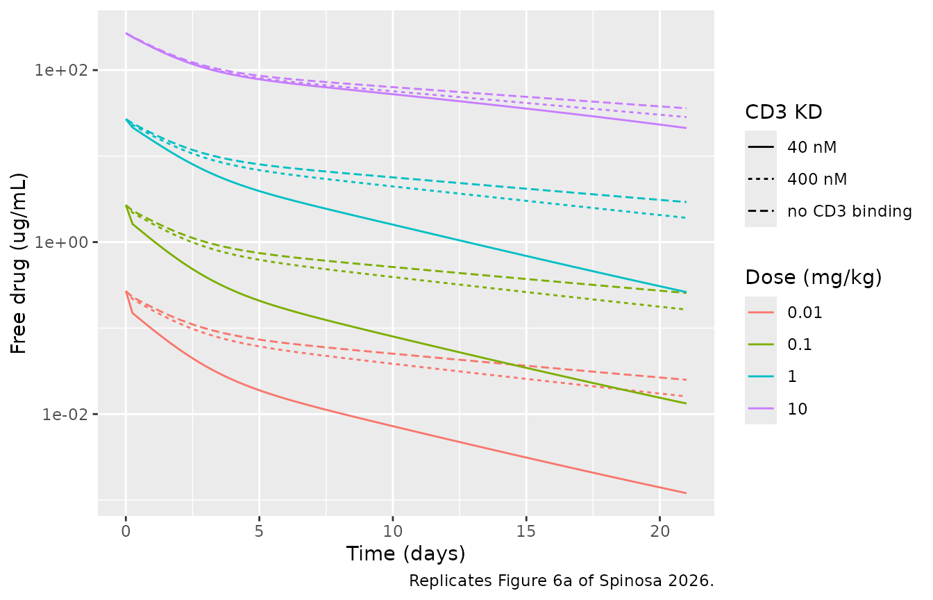
cl_share <- sim_cs3 |>
  filter(time == 21, affinity != "no CD3 binding") |>
  mutate(total = elim_ns + elim_cd20 + elim_cd3,
         NS = 100 * elim_ns / total, CD20 = 100 * elim_cd20 / total, CD3 = 100 * elim_cd3 / total) |>
  select(affinity, dose, NS, CD20, CD3)
cl_share |>
  tidyr::pivot_longer(c(NS, CD20, CD3), names_to = "route", values_to = "pct") |>
  ggplot(aes(factor(dose), pct, fill = route)) +
  geom_col() +
  facet_wrap(~affinity) +
  labs(x = "Dose (mg/kg)", y = "Share of drug cleared by day 21 (%)", fill = NULL,
       caption = "Replicates Figure 6b,c of Spinosa 2026.")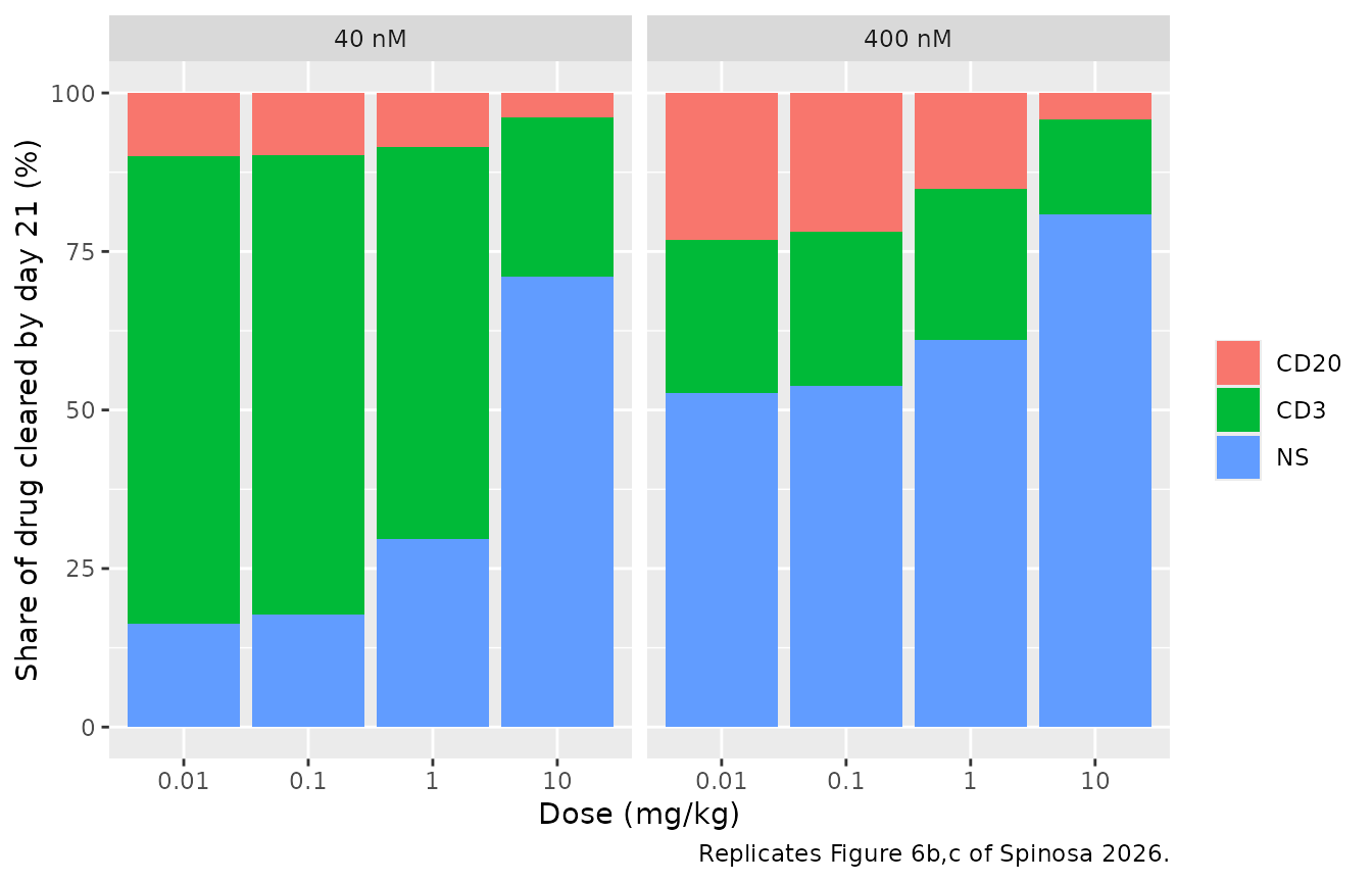
sh <- function(aff, d, col) cl_share[[col]][cl_share$affinity == aff & cl_share$dose == d]
stopifnot(
  # Moderate CD3 affinity: CD3-mediated disposition dominates below 10 mg/kg.
  all(sapply(c(0.01, 0.1, 1), sh, aff = "40 nM", col = "CD3") > 50),
  # Low CD3 affinity: nonspecific clearance dominates at every dose.
  all(sapply(c(0.01, 0.1, 1, 10), sh, aff = "400 nM", col = "NS") > 50)
)
Case Study 4: tumor-targeted bispecific versus a bivalent antibody (Figure 7)
Therapeutic-receptor occupancy (RO) at day 21 after a single IV dose, for the bispecific at effective avidities 1 to 10^6 (Figure 7c,d) and for the bivalent monospecific comparator (Figure 7e,f).
cs4_doses <- c(0.01, 0.03, 0.1, 0.3, 1, 3, 10)
grid <- tidyr::crossing(dose = cs4_doses, chi_ther = 10^(0:6)) |> mutate(id = row_number())
ev_cs4 <- bind_rows(
  grid |> mutate(time = 0, amt = dose, evid = 1),
  grid |> mutate(time = 21, amt = 0, evid = 0)
) |>
  mutate(cmt = "central") |>
  arrange(id, time, desc(evid))
ro_bs <- solve_typical(rx_tt, ev_cs4, keep = c("dose", "chi_ther"), returnType = "data.frame") |>
  filter(time == 21) |>
  select(dose, chi_ther, central = ro_ther_central, tumor = ro_ther_tumor) |>
  tidyr::pivot_longer(c(central, tumor), names_to = "location", values_to = "RO")

ggplot(ro_bs, aes(factor(dose), factor(chi_ther), fill = RO)) +
  geom_tile() +
  geom_text(aes(label = round(RO)), size = 3, colour = "white") +
  facet_wrap(~location) +
  scale_fill_viridis_c(limits = c(0, 100)) +
  labs(x = "Dose (mg/kg)", y = "Effective avidity", fill = "RO (%)",
       caption = "Replicates Figure 7c,d of Spinosa 2026.")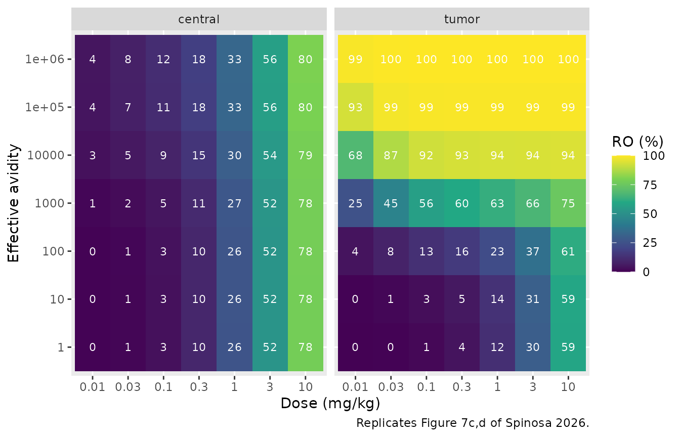
ev_bv <- bind_rows(
  tibble::tibble(id = seq_along(cs4_doses), dose = cs4_doses, time = 0, amt = cs4_doses, evid = 1),
  tibble::tibble(id = seq_along(cs4_doses), dose = cs4_doses, time = 21, amt = 0, evid = 0)
) |>
  mutate(cmt = "central") |>
  arrange(id, time, desc(evid))
ro_bv <- solve_typical(rx_bv, ev_bv, keep = "dose", returnType = "data.frame") |>
  filter(time == 21) |>
  select(dose, central = ro_ther_central, tumor = ro_ther_tumor)
knitr::kable(ro_bv |> mutate(across(c(central, tumor), round)) |>
  dplyr::rename("Dose (mg/kg)" = dose, "RO central (%)" = central, "RO tumor (%)" = tumor),
caption = "Bivalent antibody RO at day 21 (Figure 7e,f).")| Dose (mg/kg) | RO central (%) | RO tumor (%) |
|---|---|---|
| 0.01 | 13 | 6 |
| 0.03 | 29 | 15 |
| 0.10 | 54 | 35 |
| 0.30 | 74 | 58 |
| 1.00 | 89 | 79 |
| 3.00 | 96 | 91 |
| 10.00 | 99 | 97 |
ro <- function(loc, chi, d) {
  vapply(d, function(dd) ro_bs$RO[ro_bs$location == loc & ro_bs$chi_ther == chi & ro_bs$dose == dd], numeric(1))
}
stopifnot(
  # Avidity has little effect on blood RO (Figure 7c): within 15 points at 10 mg/kg.
  abs(ro("central", 1e6, 10) - ro("central", 1, 10)) < 15,
  # but drives tumor RO (Figure 7d): near-complete at 1e6, low at 1 for low doses.
  all(ro("tumor", 1e6, cs4_doses) > 95),
  all(ro("tumor", 1, c(0.01, 0.03, 0.1)) < 5),
  # At avidity 1000 the bispecific reaches > 50% tumor RO with < 40% blood RO at 0.1-1 mg/kg.
  all(ro("tumor", 1000, c(0.1, 0.3, 1)) > 50),
  all(ro("central", 1000, c(0.1, 0.3, 1)) < 40),
  # The bivalent antibody engages blood more than tumor at every dose (Figure 7e,f)
  all(ro_bv$central > ro_bv$tumor),
  # and engages blood more than the bispecific does (Figure 7e vs 7c).
  all(ro_bv$central > ro("central", 1000, cs4_doses))
)
Assumptions and deviations
- Model reduction. Each file drops the published species that stay at zero under its case study’s flags and target burden (for example, the safety and efficacy compartments when they receive no lymph flow and express no target, or membrane-receptor species when no membrane receptor is expressed). The reduction is exact; it was verified numerically against a full translation of the published SimBiology model.
- Mosunetuzumab receptor capacities. The workbook sheet “Case Study 2 Mosunetuzumab” holds 2.3e12 CD20 and 8e12 CD3 receptors per mL (3.8 and 13.3 nM), whereas Table S2 gives the fitted capacities 4.4 and 19 nM, which the “Case Study 3” sheet also uses (4.48 and 19.1 nM). Simulated with the Table S2 values, the model reproduces the central line of Figure 5d at day 40 for all three doses; the sheet’s CD3 value is the lower edge of the +/-30% band (19 x 0.7). The model therefore uses the Table S2 values.
- CD3 turnover half-life. Table S2 prints 0.7 day; the workbook runs 0.7083 day (17 h), which is used.
-
Avidity in Case Study 4. The published model
computes the effective avidity as
avid / (Vchi * cells per mL). The workbook givesavid= 1e9 for the therapeutic arm binding second and 1 for the targeting arm binding second but noVchi; the project’s defaultVchi(1.76e-8 mL/cell) would make the therapeutic-arm factor 5.7e10, contradicting the Figure 7 caption (“avidity factor held constant at 1000”). Dividing by 10^6 (the cells per mL) reproduces the caption’s 1000 and, with the same normalization, gives 1e-6 for the targeting arm. The files therefore carry the effective factors directly (chi_ther= 1000,chi_tgt= 1e-6), and with them the model reproduces the occupancy patterns of Figure 7c-f. The bivalent comparator’s factor (1000) comes from the project variant “6. AVIDITY: same cell bv mAb” (avid 1e9) under the same normalization; the paper text does not state it. - Bivalent comparator clearance. Table S4 gives 2.8 mL/kg/day for both molecules and the workbook 2.8272 for the bispecific; the bivalent file uses 2.8272 as well.
- Cytokine units. The model works in nM. The paper reports serum IL-17AA and IL-13 in pg/mL but does not give the cytokine molecular weights, so Figure 3b is reproduced in molar units. The baseline bracket uses the project variants “fit target everywhere low/high IL17” (1e-6 and 8.753e-6 nM), which span the 0.04-0.3 pg/mL range of the text. Table S1 prints the IL-17AA range as 0.04-3 pg/mL, which disagrees with the text’s 0.04-0.3 pg/mL; the model’s nominal baseline is the workbook value either way.
- Not shipped. The calibration molecules of Figure 5a-c (anti-gD, anti-gD/CD3 low and high affinity, obinutuzumab, the anti-CD20/CD3 tool molecules) are not provided as models because their affinities and clearances are not reported in the paper, its tables or the parameter workbook. Figure 7b (the affinity-ratio sweep) is not reproduced because the paper does not say which arm’s affinity was varied.
- No variability. None of the case studies estimates inter-individual variability or residual error; each file carries a fixed zero proportional error so it can be used for simulation.