Model and source
mod <- readModelDb("Kato_2021_amikacin")
mod_meta <- rxode2::rxode2(mod)$meta
#> ℹ parameter labels from comments will be replaced by 'label()'- Citation: Kato H, Parker SL, Roberts JA, Hagihara M, Asai N, Yamagishi Y, Paterson DL, Mikamo H. Population Pharmacokinetics Analysis of Amikacin Initial Dosing Regimen in Elderly Patients. Antibiotics (Basel). 2021;10(2):100. doi:10.3390/antibiotics10020100
- Description: One-compartment IV population PK model for amikacin in hospitalized elderly Japanese patients (aged 70 years and over) treated for serious infections, with clearance directly proportional to Cockcroft-Gault creatinine clearance. Estimated with the Pmetrics non-parametric adaptive grid (NPAG); the between-subject variability is a log-normal approximation of the published non-parametric distribution (Kato 2021, n = 15 patients, 33 samples).
- Article (DOI): https://doi.org/10.3390/antibiotics10020100
Kato 2021 describes amikacin in 15 hospitalized patients aged 70 years and over with a one-compartment model in which clearance is directly proportional to Cockcroft-Gault creatinine clearance (CCr). The model was estimated with the non-parametric adaptive grid (NPAG) algorithm of Pmetrics. The paper then uses Monte Carlo simulation to screen 200-2000 mg regimens given every 24, 48 or 72 h against an efficacy target (Cmax/MIC >= 8) and a safety target (Cmin < 4 mg/L). This vignette checks the packaged model against the paper’s Table 2 parameter estimates, the per-kilogram values quoted in its Discussion, and the 1080-cell probability-of-target-attainment grid of Table 3.
Population
The analysis is a single-centre retrospective therapeutic drug monitoring study at Aichi Medical University Hospital, Japan (September 2009 - February 2015). Fifteen patients aged 71-95 years (mean 80.6) were included, 9 female and 6 male. They were light (mean weight 44.8 kg, range 32.5-67.3; mean BMI 19.1) and hypoalbuminaemic (mean albumin 2.5 g/dL). Mean Cockcroft-Gault creatinine clearance was 52.9 mL/min (median 52.1, range 10.9-94.9). Infections were mostly pneumonia and bacteremia, and Pseudomonas aeruginosa was the commonest isolate. Amikacin was given at 200-1000 mg/day (mean 440 mg/day, 9.6 mg/kg/day) by 0.5-1.0 h infusion, and 33 serum concentrations (2-3 per patient, a peak and a trough) were measured (Kato 2021 Table 1, Sections 2.1-2.2 and 4.1-4.2). Patients on renal replacement therapy were excluded.
str(mod_meta$population)
#> List of 15
#>  $ species       : chr "human"
#>  $ n_subjects    : int 15
#>  $ n_studies     : int 1
#>  $ n_samples     : int 33
#>  $ age_range     : chr "71-95 years"
#>  $ age_median    : chr "80.0 years (mean 80.6 +/- 7.3)"
#>  $ weight_range  : chr "32.5-67.3 kg"
#>  $ weight_median : chr "42.6 kg (mean 44.8 +/- 8.9)"
#>  $ sex_female_pct: num 60
#>  $ race_ethnicity: chr "Japanese (single Japanese university hospital); not tabulated"
#>  $ disease_state : chr "Elderly inpatients (>= 70 years) treated with amikacin for >= 3 days: pneumonia 5, bacteremia 5, urinary tract "| __truncated__
#>  $ renal_function: chr "Cockcroft-Gault creatinine clearance mean 52.9 +/- 22.8 mL/min, median 52.1 (range 10.9-94.9); patients on inte"| __truncated__
#>  $ dose_range    : chr "Amikacin 200-1000 mg/day IV (mean 440 +/- 226 mg/day; 9.6 +/- 3.6 mg/kg/day) by 0.5-1.0 h infusion (median 0.5 "| __truncated__
#>  $ regions       : chr "Japan (Aichi Medical University Hospital)"
#>  $ notes         : chr "Single-centre retrospective therapeutic drug monitoring study, September 2009 - February 2015 (Kato 2021 Sectio"| __truncated__
Source trace
| Element | Value | Source location |
|---|---|---|
| Structure: one compartment, first-order elimination, IV infusion | – | Section 2.2 (‘the one-compartment linear model described the data adequately’); Section 4.3 |
lcl (CLs at CCr = 52.9 mL/min) |
log(2.25) L/h | Table 2, CL mean 2.25 (SD 0.78, median 2.19, CV 34.6%); abstract |
lvc (Vd) |
log(18.0) L | Table 2, V mean 18.0 (SD 3.4, median 17.1, CV 18.9%); abstract |
CL covariate model CL = CLs * (CRCL / 52.9)
|
– | Section 2.2, final-model equation |
etalcl |
log(0.346^2 + 1) = 0.113075 | Table 2, CL CV 34.6% (log-normal approximation of the NPAG distribution) |
etalvc |
log(0.189^2 + 1) = 0.035098 | Table 2, V CV 18.9% (log-normal approximation) |
propSd, addSd
|
fixed(0) | Not reported; see Assumptions and deviations |
Covariate CRCL (raw Cockcroft-Gault, mL/min) |
– | Section 4.2; Table 1 footnote |
Parameter checks against the paper
The paper’s Table 2 reports each parameter’s mean, SD and CV%.
CV% = SD / mean holds for both rows, which confirms the CV%
column describes the spread of the population distribution (a
between-subject statistic) rather than estimation precision. The
Discussion quotes the estimates per kilogram at the cohort mean weight
of 44.8 kg as 0.05 L/h/kg and 0.40 L/kg.
ini_df <- rxode2::rxode2(mod)$iniDf
#> ℹ parameter labels from comments will be replaced by 'label()'
theta <- setNames(ini_df$est, ini_df$name)
cl_typ <- exp(theta[["lcl"]])
v_typ <- exp(theta[["lvc"]])

param_check <- data.frame(
  quantity = c("CV% of CL = SD / mean", "CV% of V = SD / mean",
               "CL per kg (L/h/kg)", "V per kg (L/kg)"),
  reproduced = c(100 * 0.78 / 2.25, 100 * 3.4 / 18.0,
                 cl_typ / 44.8, v_typ / 44.8),
  published = c(34.6, 18.9, 0.05, 0.40)
)
knitr::kable(param_check, digits = 3,
caption = "Table 2 internal consistency and Discussion per-kg values.")| quantity | reproduced | published |
|---|---|---|
| CV% of CL = SD / mean | 34.667 | 34.60 |
| CV% of V = SD / mean | 18.889 | 18.90 |
| CL per kg (L/h/kg) | 0.050 | 0.05 |
| V per kg (L/kg) | 0.402 | 0.40 |
Virtual cohort
The paper does not publish individual data, so a 200-subject cohort
is drawn with creatinine clearance from a normal distribution matching
the Table 1 mean and SD (52.9 +/- 22.8 mL/min), rejecting and redrawing
values outside the observed range 10.9-94.9 mL/min. Between-subject
random effects are drawn in base R from the model’s own
omega, so the cohort is identical on every rxode2 build,
and they are passed to the typical-value model as data columns.
omega <- rxode2::rxode2(mod)$omega
#> ℹ parameter labels from comments will be replaced by 'label()'
mod_typ <- rxode2::zeroRe(mod)
#> ℹ parameter labels from comments will be replaced by 'label()'

draw_crcl <- function(n, mean = 52.9, sd = 22.8, lo = 10.9, hi = 94.9) {
  out <- numeric(0)
  while (length(out) < n) {
    x <- rnorm(2 * n, mean, sd)
    out <- c(out, x[x >= lo & x <= hi])
  }
  out[seq_len(n)]
}

set.seed(2021)
n_sub <- 200
cohort <- data.frame(
  id = seq_len(n_sub),
  CRCL = draw_crcl(n_sub),
  etalcl = rnorm(n_sub, 0, sqrt(omega["etalcl", "etalcl"])),
  etalvc = rnorm(n_sub, 0, sqrt(omega["etalvc", "etalvc"]))
)
summary(cohort$CRCL)
#>    Min. 1st Qu.  Median    Mean 3rd Qu.    Max.
#>   10.91   38.11   51.80   51.81   64.45   93.03
Simulation
Each virtual patient receives a single 400 mg dose (the Table 1 median daily dose) as a 0.5 h infusion (the Table 1 median infusion time), observed on a dense grid out to 48 h, from which PKNCA extrapolates to infinity. The grid stops at 48 h, and the solver tolerances are tightened, because fast-clearing subjects otherwise fall to numerical-noise concentrations (including tiny negative values) that PKNCA cannot use.
obs_times <- sort(unique(c(0, 0.25, 0.5, 0.75, 1, 1.5, 2, 3, 4, 6, 8, 12,
                           16, 24, 30, 36, 42, 48)))
dose_rows <- cohort |>
  mutate(time = 0, amt = 400, rate = 400 / 0.5, evid = 1L, cmt = "central")
obs_rows <- tidyr::crossing(cohort, time = obs_times) |>
  mutate(amt = 0, rate = 0, evid = 0L, cmt = "central")
events <- bind_rows(dose_rows, obs_rows) |>
  arrange(id, time, desc(evid)) |>
  select(id, time, amt, rate, evid, cmt, CRCL, etalcl, etalvc)

sim <- rxode2::rxSolve(mod_typ, events = events, returnType = "data.frame",
                       keep = "CRCL", atol = 1e-12, rtol = 1e-10)
#> ℹ omega/sigma items treated as zero: 'etalcl', 'etalvc'
#> Warning: multi-subject simulation without without 'omega'
stopifnot(all(sim$Cc >= 0))
sim_obs <- sim |> filter(!is.na(Cc))
Solver check against the closed-form solution
With the random effects supplied as data, each simulated profile must equal the analytical one-compartment infusion solution for that subject’s own clearance and volume. Both sides use the same drawn parameters, so the only difference is numerical error and the bound is tight.
closed_form <- function(t, dose, tinf, cl, v) {
  k <- cl / v
  r0 <- dose / tinf
  ifelse(t <= tinf,
         r0 / cl * (1 - exp(-k * t)),
         r0 / cl * (1 - exp(-k * tinf)) * exp(-k * (t - tinf)))
}
chk <- sim_obs |>
  select(id, time, Cc, CRCL) |>
  left_join(cohort |> select(id, etalcl, etalvc), by = "id") |>
  mutate(
    cl_i = cl_typ * exp(etalcl) * CRCL / 52.9,
    v_i = v_typ * exp(etalvc),
    Cc_cf = closed_form(time, 400, 0.5, cl_i, v_i)
  ) |>
  # Relative error is compared above 0.01 mg/L (far below the 0.8 mg/L assay
  # limit), where the solver's absolute tolerance does not dominate.
  filter(time > 0, Cc_cf > 0.01)
max_rel_err <- max(abs(chk$Cc - chk$Cc_cf) / chk$Cc_cf)
max_rel_err
#> [1] 1.218209e-09
stopifnot(max_rel_err < 1e-4)
Simulated profiles
sim_obs |>
  mutate(crcl_band = cut(CRCL, c(0, 30, 60, 100),
                         labels = c("CRCL < 30", "CRCL 30-60", "CRCL > 60"))) |>
  group_by(crcl_band, time) |>
  summarise(
    Q05 = quantile(Cc, 0.05), Q50 = median(Cc), Q95 = quantile(Cc, 0.95),
    .groups = "drop"
  ) |>
  filter(time > 0) |>
  ggplot(aes(time, Q50, colour = crcl_band, fill = crcl_band)) +
  geom_ribbon(aes(ymin = Q05, ymax = Q95), alpha = 0.15, colour = NA) +
  geom_line() +
  scale_y_log10() +
  labs(x = "Time after start of infusion (h)",
       y = "Amikacin serum concentration (mg/L)",
       colour = NULL, fill = NULL,
       title = "Single 400 mg dose over 0.5 h, 200 virtual patients",
       subtitle = "Median and 5th-95th percentiles by creatinine-clearance band") +
  theme_minimal()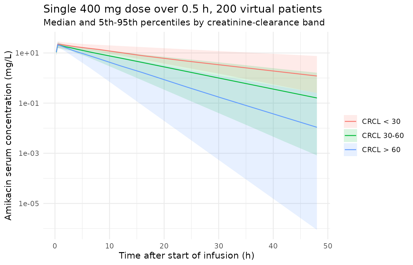
PKNCA validation
The paper reports no non-compartmental summary, so the NCA is checked
against the model’s own identity: for linear IV kinetics,
AUC0-inf = Dose / CL for each subject’s individual
clearance.
nca_conc <- sim_obs |>
  mutate(treatment = "400 mg single dose") |>
  select(id, time, Cc, treatment) |>
  as.data.frame()
nca_dose <- dose_rows |>
  mutate(treatment = "400 mg single dose") |>
  select(id, time, amt, treatment) |>
  as.data.frame()

conc_obj <- PKNCA::PKNCAconc(nca_conc, Cc ~ time | treatment + id,
                             concu = "mg/L", timeu = "h")
dose_obj <- PKNCA::PKNCAdose(nca_dose, amt ~ time | treatment + id,
                             doseu = "mg")
intervals <- data.frame(
  start = 0, end = Inf,
  cmax = TRUE, tmax = TRUE, aucinf.obs = TRUE, half.life = TRUE
)
nca_res <- PKNCA::pk.nca(PKNCA::PKNCAdata(conc_obj, dose_obj,
                                          intervals = intervals))
knitr::kable(summary(nca_res), caption = "Simulated single-dose NCA (PKNCA).")| Interval Start | Interval End | treatment | N | Cmax (mg/L) | Tmax (h) | Half-life (h) | AUCinf,obs (h*mg/L) |
|---|---|---|---|---|---|---|---|
| 0 | Inf | 400 mg single dose | 200 | 20.9 [17.3] | 0.500 [0.500, 0.500] | 7.47 [5.19] | 193 [61.4] |
auc_chk <- as.data.frame(nca_res) |>
  filter(PPTESTCD == "aucinf.obs") |>
  mutate(id = as.integer(id)) |>
  left_join(cohort, by = "id") |>
  mutate(
    cl_i = cl_typ * exp(etalcl) * CRCL / 52.9,
    pct_diff = 100 * (PPORRES - 400 / cl_i) / (400 / cl_i)
  )
summary(auc_chk$pct_diff)
#>       Min.    1st Qu.     Median       Mean    3rd Qu.       Max.
#> -0.1293492 -0.0137004 -0.0072202 -0.0118259 -0.0028998 -0.0002025
stopifnot(
  abs(median(auc_chk$pct_diff)) < 2,
  quantile(abs(auc_chk$pct_diff), 0.9) < 5
)
Replicate Table 3: probability of target attainment
Table 3 of Kato 2021 marks, for each regimen (200-2000 mg every 24,
48 or 72 h) and creatinine clearance (10-90 mL/min), whether at least
90% of 1000 simulated patients met each target:
Cmin < 4 mg/L and Cmax/MIC >= 8 for MICs
of 4, 8 and 16 mg/L. That is 3 x 9 x 10 x 4 = 1080 binary cells. The
grid below was transcribed by the maintainers from the three raster
panels of Table 3, by classifying each printed glyph as +
or -.
Section 4.6 of the paper defines Cmax as the concentration 1 h after the start of a 30 min infusion and Cmin as the concentration 23.5, 47.5 or 71.5 h after the start of infusion for the q24h, q48h and q72h regimens. It does not say which dose the Cmax refers to. The primary reading below takes both from the first dose; a sensitivity reading takes Cmax after the tenth dose, which is close to steady state.
t3_rows <- list(
  q24h = c(
    "---- ---- -+-- -+-- -++- -++- -++- -++- -++- -+++",
    "---- ---- -+-- -+-- -+-- -++- -++- -++- -++- -++-",
    "+--- ---- -+-- -+-- -+-- -++- -++- -++- -++- -++-",
    "+--- ---- ---- -+-- -+-- -+-- -++- -++- -++- -++-",
    "+--- ---- ---- -+-- -+-- -+-- -++- -++- -++- -++-",
    "+--- +--- ---- -+-- -+-- -+-- -++- -++- -++- -++-",
    "+--- +--- +--- -+-- -+-- -+-- -+-- -++- -++- -++-",
    "+--- +--- +--- ++-- -+-- -+-- -+-- -++- -++- -++-",
    "+--- +--- +--- ++-- ++-- -+-- -+-- -++- -++- -++-"
  ),
  q48h = c(
    "---- ---- -+-- -+-- -+-- -++- -++- -++- -++- -++-",
    "+--- ---- ---- -+-- -+-- -+-- -++- -++- -++- -++-",
    "+--- +--- ---- -+-- -+-- -+-- -++- -++- -++- -++-",
    "+--- +--- +--- ++-- -+-- -+-- -+-- -++- -++- -++-",
    "+--- +--- +--- ++-- ++-- ++-- ++-- -++- -++- -++-",
    "+--- +--- +--- ++-- ++-- ++-- ++-- ++-- +++- +++-",
    "+--- +--- +--- ++-- ++-- ++-- ++-- ++-- +++- +++-",
    "+--- +--- +--- +--- ++-- ++-- ++-- ++-- +++- +++-",
    "+--- +--- +--- +--- ++-- ++-- ++-- ++-- +++- +++-"
  ),
  q72h = c(
    "+--- ---- -+-- -+-- -+-- -++- -++- -++- -++- -++-",
    "+--- +--- ---- -+-- -+-- -+-- -++- -++- -++- -++-",
    "+--- +--- +--- ++-- ++-- -+-- -+-- -++- -++- -++-",
    "+--- +--- +--- ++-- ++-- ++-- ++-- ++-- +++- +++-",
    "+--- +--- +--- +--- ++-- ++-- ++-- ++-- +++- +++-",
    "+--- +--- +--- +--- ++-- ++-- ++-- ++-- +++- +++-",
    "+--- +--- +--- +--- ++-- ++-- ++-- ++-- +++- +++-",
    "+--- +--- +--- +--- ++-- ++-- ++-- ++-- +++- +++-",
    "+--- +--- +--- +--- ++-- ++-- ++-- ++-- +++- +++-"
  )
)
targets <- c("cmin", "mic4", "mic8", "mic16")
paper_t3 <- bind_rows(lapply(names(t3_rows), function(iv) {
  bind_rows(lapply(seq_along(t3_rows[[iv]]), function(i) {
    glyphs <- strsplit(gsub(" ", "", t3_rows[[iv]][i]), "")[[1]]
    stopifnot(length(glyphs) == 40)
    data.frame(
      interval = iv,
      crcl = 10 * i,
      dose = rep(seq(200, 2000, 200), each = 4),
      target = rep(targets, times = 10),
      paper = as.integer(glyphs == "+")
    )
  }))
}))
stopifnot(nrow(paper_t3) == 1080)
The 1080 cells are simulated with 200 patients per interval and creatinine clearance (the paper used 1000), sharing one set of base-R random-effect draws. Because the model is linear, every regimen is a dose multiple of a single 1000 mg solve.
n_pta <- 200
set.seed(20210120)
pta_eta <- data.frame(
  sub = seq_len(n_pta),
  etalcl = rnorm(n_pta, 0, sqrt(omega["etalcl", "etalcl"])),
  etalvc = rnorm(n_pta, 0, sqrt(omega["etalvc", "etalvc"]))
)
pta_design <- tidyr::crossing(tau = c(24, 48, 72), crcl = seq(10, 90, 10),
                              pta_eta) |>
  mutate(id = row_number())

pta_dose <- pta_design |>
  mutate(time = 0, amt = 1000, rate = 1000 / 0.5, ii = tau, addl = 9L,
         evid = 1L)
pta_obs <- bind_rows(
  pta_design |> mutate(time = 1, what = "cmax_first"),
  pta_design |> mutate(time = tau - 0.5, what = "cmin"),
  pta_design |> mutate(time = 9 * tau + 1, what = "cmax_10th")
) |>
  mutate(amt = 0, rate = 0, ii = 0, addl = 0L, evid = 0L)
pta_events <- bind_rows(pta_dose, pta_obs) |>
  mutate(cmt = "central", CRCL = crcl) |>
  arrange(id, time, desc(evid)) |>
  select(id, time, amt, rate, ii, addl, evid, cmt, CRCL, etalcl, etalvc)

pta_sim <- rxode2::rxSolve(mod_typ, events = pta_events,
                           returnType = "data.frame") |>
  filter(!is.na(Cc)) |>
  select(id, time, Cc) |>
  left_join(pta_obs |> select(id, time, what, tau, crcl), by = c("id", "time"))
#> ℹ omega/sigma items treated as zero: 'etalcl', 'etalvc'
#> Warning: multi-subject simulation without without 'omega'
stopifnot(nrow(pta_sim) == 3 * nrow(pta_design))

pta_wide <- pta_sim |>
  select(id, tau, crcl, what, Cc) |>
  tidyr::pivot_wider(names_from = what, values_from = Cc)

pta_grid <- function(wide, cmax_col) {
  bind_rows(lapply(seq(200, 2000, 200), function(d) {
    wide |>
      mutate(cmax = .data[[cmax_col]] * d / 1000,
             cmin_d = cmin * d / 1000) |>
      group_by(tau, crcl) |>
      summarise(cmin = mean(cmin_d < 4), mic4 = mean(cmax / 4 >= 8),
                mic8 = mean(cmax / 8 >= 8), mic16 = mean(cmax / 16 >= 8),
                .groups = "drop") |>
      mutate(dose = d)
  })) |>
    tidyr::pivot_longer(c(cmin, mic4, mic8, mic16), names_to = "target",
                        values_to = "pta") |>
    mutate(interval = paste0("q", tau, "h"), sim = as.integer(pta >= 0.9)) |>
    select(interval, crcl, dose, target, pta, sim)
}
cmp_first <- inner_join(paper_t3, pta_grid(pta_wide, "cmax_first"),
                        by = c("interval", "crcl", "dose", "target"))
cmp_10th <- inner_join(paper_t3, pta_grid(pta_wide, "cmax_10th"),
                       by = c("interval", "crcl", "dose", "target"))
stopifnot(nrow(cmp_first) == 1080, nrow(cmp_10th) == 1080)
agree_tab <- function(cmp, label) {
  cmp |>
    group_by(target) |>
    summarise(agreement = mean(sim == paper), .groups = "drop") |>
    bind_rows(data.frame(target = "all", agreement = mean(cmp$sim == cmp$paper))) |>
    mutate(reading = label)
}
agreement <- bind_rows(
  agree_tab(cmp_first, "Cmax after the first dose"),
  agree_tab(cmp_10th, "Cmax after the tenth dose")
)
agreement |>
  tidyr::pivot_wider(names_from = reading, values_from = agreement) |>
  dplyr::rename("Target" = target) |>
  knitr::kable(digits = 3,
caption = "Fraction of Table 3 cells whose >= 90% PTA flag is reproduced.")| Target | Cmax after the first dose | Cmax after the tenth dose |
|---|---|---|
| cmin | 0.930 | 0.930 |
| mic16 | 0.996 | 0.981 |
| mic4 | 0.959 | 0.985 |
| mic8 | 0.911 | 0.963 |
| all | 0.949 | 0.965 |
cmp_first |>
  mutate(
    status = case_when(
      sim == paper & paper == 1 ~ "both >= 90%",
      sim == paper ~ "both < 90%",
      sim == 1 ~ "simulated only",
      TRUE ~ "paper only"
    ),
    target = factor(target, targets,
                    c("Cmin < 4", "Cmax/MIC >= 8, MIC 4",
                      "Cmax/MIC >= 8, MIC 8", "Cmax/MIC >= 8, MIC 16"))
  ) |>
  ggplot(aes(factor(dose), factor(crcl), fill = status)) +
  geom_tile(colour = "white") +
  facet_grid(target ~ interval) +
  scale_fill_manual(values = c("both >= 90%" = "#2c7fb8",
                               "both < 90%" = "#d9d9d9",
                               "simulated only" = "#fdae61",
                               "paper only" = "#d7191c")) +
  labs(x = "Dose (mg)", y = "Creatinine clearance (mL/min)", fill = NULL,
       title = "Replicates Table 3 of Kato 2021 (first-dose reading)") +
  theme_minimal() +
  theme(axis.text.x = element_text(angle = 90, vjust = 0.5, size = 6),
        axis.text.y = element_text(size = 6),
        legend.position = "bottom")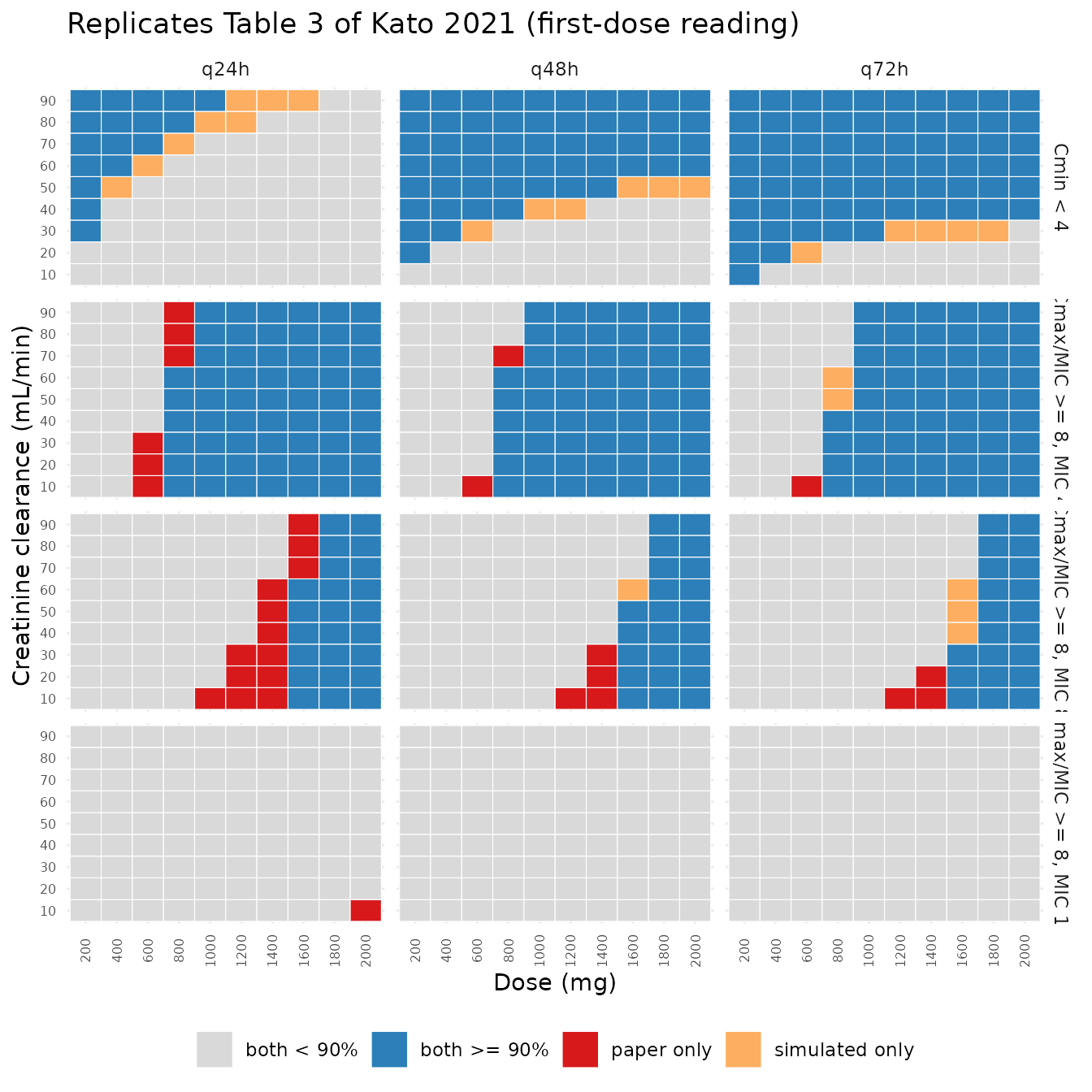
The two readings agree with the paper equally well on the trough target, since the trough is always taken after the first dose. For the Cmax targets the readings differ mainly at q24h, the only interval with appreciable accumulation, where the paper’s flags sit closer to the tenth-dose reading:
cmax_by_interval <- bind_rows(
  cmp_first |> mutate(reading = "first dose"),
  cmp_10th |> mutate(reading = "tenth dose")
) |>
  filter(target != "cmin") |>
  group_by(interval, reading) |>
  summarise(agreement = mean(sim == paper), .groups = "drop") |>
  tidyr::pivot_wider(names_from = reading, values_from = agreement)
cmax_by_interval |>
  dplyr::rename("Interval" = interval,
                "Cmax agreement, first dose" = `first dose`,
                "Cmax agreement, tenth dose" = `tenth dose`) |>
knitr::kable(digits = 3, caption = "Agreement on the three Cmax/MIC targets by interval.")| Interval | Cmax agreement, first dose | Cmax agreement, tenth dose |
|---|---|---|
| q24h | 0.926 | 0.963 |
| q48h | 0.974 | 0.985 |
| q72h | 0.967 | 0.981 |
q24 <- cmax_by_interval |> filter(interval == "q24h")
stopifnot(q24$`tenth dose` > q24$`first dose`)
The regimens the paper recommends (Table 5: 1800 mg q72h at CCr 40-50 mL/min and 1800 mg q48h at CCr 60-90 mL/min) meet both the trough target and the MIC 8 mg/L efficacy target in the simulation:
recommended <- data.frame(
  interval = c("q72h", "q72h", rep("q48h", 4)),
  crcl = c(40, 50, 60, 70, 80, 90),
  dose = 1800
)
rec_chk <- cmp_first |>
  filter(target %in% c("cmin", "mic8")) |>
  inner_join(recommended, by = c("interval", "crcl", "dose")) |>
  select(interval, crcl, target, pta, paper) |>
  tidyr::pivot_wider(names_from = target, values_from = c(pta, paper))
rec_chk |>
  dplyr::rename("Interval" = interval, "CCr (mL/min)" = crcl,
                "PTA Cmin < 4 (sim)" = pta_cmin,
                "PTA Cmax/MIC >= 8, MIC 8 (sim)" = pta_mic8,
                "Paper Cmin flag" = paper_cmin,
                "Paper MIC 8 flag" = paper_mic8) |>
knitr::kable(digits = 3, caption = "Table 5 recommended regimens.")| Interval | CCr (mL/min) | PTA Cmin < 4 (sim) | PTA Cmax/MIC >= 8, MIC 8 (sim) | Paper Cmin flag | Paper MIC 8 flag |
|---|---|---|---|---|---|
| q48h | 60 | 0.975 | 0.975 | 1 | 1 |
| q48h | 70 | 0.990 | 0.975 | 1 | 1 |
| q48h | 80 | 0.995 | 0.975 | 1 | 1 |
| q48h | 90 | 1.000 | 0.970 | 1 | 1 |
| q72h | 40 | 0.985 | 0.975 | 1 | 1 |
| q72h | 50 | 0.990 | 0.975 | 1 | 1 |
stopifnot(all(rec_chk$pta_cmin >= 0.9), all(rec_chk$pta_mic8 >= 0.9),
          all(rec_chk$paper_cmin == 1), all(rec_chk$paper_mic8 == 1))
The gates assert an overall agreement of at least 90%, and at least 85% for each target, under the first-dose reading. A mutation control checks that the comparison is not vacuous: every concentration is halved, as a two-fold error in volume or dose unit would do, and the agreement must then fall below 80%.
cmp_mut <- cmp_first |>
  select(interval, crcl, dose, target, paper) |>
  inner_join(
    pta_grid(mutate(pta_wide, cmax_first = cmax_first / 2, cmin = cmin / 2),
             "cmax_first"),
    by = c("interval", "crcl", "dose", "target")
  )
mutated_agreement <- mean(cmp_mut$sim == cmp_mut$paper)
mutated_agreement
#> [1] 0.7592593

first_agree <- agreement |> filter(reading == "Cmax after the first dose")
stopifnot(
  first_agree$agreement[first_agree$target == "all"] >= 0.90,
  all(first_agree$agreement[first_agree$target != "all"] >= 0.85),
  mutated_agreement < 0.80
)
With the concentrations halved, the agreement falls to 76%, against 95% for the model as published.
Assumptions and deviations
-
Log-normal approximation of a non-parametric
distribution. Pmetrics NPAG estimates a discrete joint
distribution of support points, which the paper does not publish. Table
2 summarises it by mean, SD, median and CV% per parameter. The model
uses the mean as the typical value (as the abstract and Section 2.2 do)
and converts each CV% to a log-normal variance with
omega^2 = log(CV^2 + 1). The two random effects are independent because no correlation is reported. Because the typical value is the median of a log-normal, the model’s medians (2.25 L/h, 18.0 L) sit above the published medians (2.19 L/h, 17.1 L) and its means sit above the published means. The shape of the discrete NPAG distribution is not captured, which is the expected source of the remaining disagreement in the Table 3 cells near the 90% threshold. -
Residual error not reported. Neither the Pmetrics
assay-error polynomial (C0-C3) nor the gamma or lambda noise term is
reported. Both residual terms are therefore
fixed(0), so simulations from this model carry no measurement error. The paper’s Table 3 targets are defined on the simulated concentrations themselves, so this does not affect the replication above. -
Reference creatinine clearance. The final-model
equation in Section 2.2 is
CL = CLs x (CCr/52.9), where 52.9 mL/min is the Table 1 cohort mean. The same section’s prose says CCr was normalized to ‘the median value of the study population of 52.1 mL/min’ (the Table 1 median). The printed equation is used. The two differ by 1.5% in clearance at any given CCr. - Table 2 ‘Var’ column. The printed variances (2.19 for CL, 17.1 for V) repeat the median column and are not the squared SDs (0.61 and 11.6). They are not used; the CV% column (which matches SD / mean) is used instead.
-
Table 3 transcription and Cmax timing. Table 3 is
printed as raster images. The maintainers transcribed its 1080
+/-cells by classifying the glyphs in the embedded images; every row yielded exactly 40 cells. The paper does not say which dose the simulated Cmax follows. The first-dose reading is used for the gates and the tenth-dose reading is shown for comparison. The simulation uses 200 patients per creatinine clearance and interval rather than the paper’s 1000. - Not reproduced. The Figure 1 diagnostics and visual predictive check need the individual data, which are not published. The fractional target attainment of Table 4 needs the EUCAST P. aeruginosa MIC distribution the authors used, which is not given in the paper.
- Covariate range. The model was fit to CCr of 10.9-94.9 mL/min in patients aged 70 years and over, with no patient on renal replacement therapy. Clearance is proportional to CCr with no non-renal intercept, so it approaches zero as CCr approaches zero; do not extrapolate far below the observed range.