Warfarin/INR from QSP model reduction (Falkenhagen 2023)

Model and source

• Citation: Falkenhagen U, Knoechel J, Kloft C, Huisinga W. Deriving mechanism-based pharmacodynamic models by reducing quantitative systems pharmacology models: An application to warfarin. CPT Pharmacometrics Syst Pharmacol. 2023;12(4):432-443. doi:10.1002/psp4.12903. Reduced in vivo ODE system from Supplementary Material Section S5 (Eqs S27-S29); INR power law from Equation (13); genotype parameters from Supplementary Table S1; steady-state parameter interdependencies from Supplementary Material Section S2 (Eq S3). Numeric values of the reference parameterization are inherited from the underlying QSP model: Wajima T, Isbister GK, Duffull SB. A comprehensive model for the humoral coagulation network in humans. Clin Pharmacol Ther. 2009;86(3):290-298. doi:10.1038/clpt.2009.87, as implemented in the authors’ own supplemental code archive doi:10.5281/zenodo.7417886.
• Description: QSP-derived mechanism-based warfarin/INR pharmacodynamic model (Falkenhagen 2023). Obtained by systematically reducing the 62-ODE / 174-parameter Wajima 2009 blood-coagulation quantitative systems pharmacology model down to 6 ODEs and 11 structural parameters, while guaranteeing under 10% relative INR error for at least 95% of a diverse virtual population. One-compartment oral warfarin PK inhibits vitamin K hydroquinone (VKH2) synthesis through an Imax function; VKH2 in turn drives the synthesis of coagulation Factors II, VII, and X, each modelled as a turnover pool holding its own pre-stimulus steady state. The INR is recovered algebraically as a power law in the product of the three relative factor concentrations, INR = INR0 * (II/II0 * VII/VII0 * X/X0)^gamma with gamma = -0.1975. CYP2C9 1/2/*3 allele counts set warfarin clearance and VKORC1 -1639 G/A allele counts set IC50, both as per-allele sums. All parameter values are the Wajima 2009 reference parameterization carried through the reduction; no parameter was estimated from clinical data in this paper.
• Article: https://doi.org/10.1002/psp4.12903
• Supporting information (Sections S1-S7, Table S1): https://doi.org/10.1002/psp4.12903
• Authors’ supplemental MATLAB code archive: https://doi.org/10.5281/zenodo.7417886

This model is unusual for the library in that it was not fitted to clinical data. It is the published end-product of a systematic, largely automated model-reduction algorithm applied to the Wajima 2009 blood-coagulation quantitative systems pharmacology (QSP) model. The reduction took a system of 62 ODEs and 174 parameters down to 6 ODEs and 11 structural parameters, subject to a hard accuracy constraint: the reduced model must reproduce the full QSP model’s INR to within 10% relative error for at least 95% of a diverse virtual population (Equation 7).

Two scenarios of the QSP model had to be reduced (Figure 3a):

1. the in vivo scenario, describing warfarin’s effect on the circulating coagulation factors, and
2. the in vitro scenario, describing the prothrombin-time (PT) test performed on a drawn blood sample.

The in vitro reduction collapsed to purely linear ODEs with an analytic solution (Supplementary Section S4), and that solution showed that fibrin, and hence PT and INR, depends on the warfarin-sensitive coagulation factors only through their product II * VII * X (Equation 12). That insight is what makes the single algebraic power law of Equation 13 sufficient, and it is the reason only the in vivo ODE system is carried in this model file.

Population

The “population” behind this model is an in silico virtual population of 1000 individuals, not a clinical cohort. It exists to define the parameter region over which the reduction is certified accurate, and it combines two sources of variability:

• Covariate-explained variability from genotype. Warfarin clearance depends on the CYP2C9 diplotype and warfarin sensitivity (IC50) on the VKORC1 -1639 G/A diplotype, each entering as a per-allele sum, CL^{a/b} = CL^a + CL^b and IC50^{ab} = IC50^a + IC50^b (Supplementary Equation S1). Genotypes were assigned deterministically so that allele frequencies matched those of the Warfarin Genetics (WARG) study as reported by Hamberg 2010: CYP2C9 *1 0.815, *2 0.112, *3 0.073; VKORC1 -1639 G 0.608, A 0.392 (Supplementary Table S1).
• Unexplained random variability, assumed rather than estimated: an independent log-normal distribution with 40% CV on every parameter and initial value, q_j ~ logN(log(q_ref_j), 0.4^2) (Equation 3, Supplementary Equation S2), drawn by Latin hypercube sampling. Parameter variability was taken as uncorrelated for lack of knowledge of the correlation structure (Discussion).

Dosing in the reduction scenario was 4 mg orally once daily for 30 days, reduced to 1 mg once daily for those virtual individuals whose steady-state INR under 4 mg would exceed 4, so as to keep the INR in a clinically relevant range.

The same information is available programmatically via readModelDb("Falkenhagen_2023_warfarin_qsp")()$population.

Source trace

Every ini() entry in inst/modeldb/specificDrugs/Falkenhagen_2023_warfarin_qsp.R carries an in-file comment naming its origin. They are collected here for review.

Structural parameters

Parameter	Value	Source location
lka (ka_warf)	1.0 1/h	Wajima 2009 reference value; Zenodo code archive Wajima2009BloodCoagulation_parameters.m
lvc (Vd_warf)	10 L	Wajima 2009 reference value; Zenodo code archive
lkel (ke_warf, *1/*1)	0.02 1/h	Derived in-source as Cl_Warf/Vd_Warf = 0.2/10; Zenodo code archive
lcl_cyp2c9_s1	0.1000 L/h per *1 allele	Supplementary Table S1
lcl_cyp2c9_s2	0.0505 L/h per *2 allele	Supplementary Table S1
lcl_cyp2c9_s3	0.0243 L/h per *3 allele	Supplementary Table S1
lic50_vkorc1_g	0.1700 mg/L per -1639G allele	Supplementary Table S1
lic50_vkorc1_a	0.0796 mg/L per -1639A allele	Supplementary Table S1
limax (Imax)	1	Wajima 2009 reference (lmax); Zenodo code archive
lkdeg_vk2 (deg_VK2)	0.0228 1/h	Wajima 2009 reference; Zenodo code archive
lkdeg_ii (deg_II)	0.010 1/h	Wajima 2009 reference; half-life 69.3 h matches the “~69 h” in Results
lkdeg_vii (deg_VII)	0.12 1/h	Wajima 2009 reference; half-life 5.8 h matches the “~6 h” in Results
lkdeg_x (deg_X)	0.018 1/h	Wajima 2009 reference; half-life 38.5 h matches the “~39 h” in Results
gamma	-0.1975	Equation (13); slope of the log-log fit in Figure 4
le0 (INR0)	1	INR = PT/PT_ref (Equation 1); Figure 6 profiles start at 1
bl_vk (VK(0))	1.0 rel. units	Wajima 2009 reference initial value; Zenodo code archive
bl_vkh2 (VKH2(0))	0.1 rel. units	Wajima 2009 reference initial value; Zenodo code archive
bl_ii (II(0))	1394.4 nmol/L	Wajima 2009 reference initial value; Zenodo code archive
bl_vii (VII(0))	10.0 nmol/L	Wajima 2009 reference initial value; Zenodo code archive
bl_x (X(0))	174.3 nmol/L	Wajima 2009 reference initial value; Zenodo code archive
all eta* variances	0.16 (= 0.4^2)	Equation (3) / Supplementary Equation S2
addSd	0 (fixed)	Not reported; the model was never fitted to data

Equations

Equation	Source location
d/dt(depot) = -ka * depot	Supplementary Equation S27 (first line)
d/dt(central) = ka * depot - kel * central	Supplementary Equation S27 (second line), rewritten on the amount scale
d/dt(vkh2) = deg_VK2 * VK(0) * (1 - Imax*Cc/(IC50+Cc)) - deg_VKH2 * vkh2	Supplementary Equation S27 (third line)
d/dt(factor_ii) = deg_II * II(0) * vkh2/VKH2(0) - deg_II * factor_ii	Supplementary Equation S27
d/dt(factor_vii) = deg_VII * VII(0) * vkh2/VKH2(0) - deg_VII * factor_vii	Supplementary Equation S28
d/dt(factor_x) = deg_X * X(0) * vkh2/VKH2(0) - deg_X * factor_x	Supplementary Equation S29
deg_VKH2 = deg_VK2 * VK(0)/VKH2(0) (derived, not free)	Supplementary Section S2
INR = INR0 * (II/II0 * VII/VII0 * X/X0)^gamma	Equation (13)
CL = CL^a + CL^b, IC50 = IC50^a + IC50^b	Supplementary Equation S1

Note the deliberate reparameterisation of the PK: Supplementary Equation S27 writes the central compartment on the concentration scale, dC_warf/dt = (ka/Vd)*A_warf - ke*C_warf. The model file multiplies through by Vd so that central carries an amount (the nlmixr2 convention) and Cc <- central/vc. The two forms are algebraically identical.

Dimensional analysis

Mechanistic models mix units freely, so each ODE term is checked explicitly.

Term	Units	Result
ka * depot	(1/h) * mg	mg/h = d/dt(depot)
kel * central	(1/h) * mg	mg/h = d/dt(central)
Cc = central/vc	mg / L	mg/L, same units as ic50 (mg/L), so Cc/(ic50+Cc) is unitless
deg_VK2 * vk_base	(1/h) * rel	rel/h = d/dt(vkh2)
deg_VKH2 * vkh2	(1/h) * rel	rel/h
deg_II * ii_base * (vkh2/vkh2_base)	(1/h) * (nmol/L) * unitless	nmol/L/h = d/dt(factor_ii)
rel_ii * rel_vii * rel_x	unitless^3	unitless, so (...)^gamma is well defined
INR	unitless * unitless^gamma	unitless

The vitamin K states VK and VKH2 are in the QSP model’s relative vitamin-K units. They never leave the model in absolute form: VK(0) appears only in the product deg_VK2 * VK(0), and VKH2 appears only as the ratio vkh2/VKH2(0). Supplementary Section S6 makes this explicit, which is why the reduced model has 11 rather than 16 identifiable quantities.

mod  <- readModelDb("Falkenhagen_2023_warfarin_qsp")
modt <- rxode2::zeroRe(mod)   # typical-value (no IIV) version for deterministic replication

# Build an event table for one warfarin regimen and one genotype.
# Observation rows use cmt = "central" (an actual ODE state) so rxode2
# returns the algebraic observables (Cc, INR, rel_vii, ...) as columns.
make_events <- function(s1, s2, s3, g, dose = 4, until = 720, by = 6,
                        id = 1L, label = NA_character_) {
  ev <- rxode2::et(amt = dose, ii = 24, until = until, cmt = "depot")
  ev <- rxode2::et(ev, seq(0, until, by = by), cmt = "central")
  d  <- as.data.frame(ev)
  d$id <- id
  d$CYP2C9_S1_COUNT    <- s1
  d$CYP2C9_S2_COUNT    <- s2
  d$CYP2C9_S3_COUNT    <- s3
  d$VKORC1_1639G_COUNT <- g
  d$genotype <- label
  d
}

cyp_diplotypes <- tibble::tribble(
  ~genotype, ~s1, ~s2, ~s3,
  "*1/*1",     2,   0,   0,
  "*1/*2",     1,   1,   0,
  "*1/*3",     1,   0,   1,
  "*2/*2",     0,   2,   0,
  "*2/*3",     0,   1,   1,
  "*3/*3",     0,   0,   2
)

# knitr::kable emits markdown, which would swallow the "*" of star-allele
# names ("*1/*1" renders as "1/1"). Escape them for table display only;
# ggplot legends take the raw strings.
esc_star <- function(x) gsub("*", "\\*", x, fixed = TRUE)

Validation 1: pre-stimulus steady state

The reduction is built on the requirement (Supplementary Section S2) that the untreated system sit exactly at its pre-stimulus steady state: the synthesis constants are defined as k_syn,j = k_deg,j * x0_j, and deg_VKH2 is defined as deg_VK2 * VK(0)/VKH2(0). If those interdependencies were transcribed incorrectly, the drug-free model would drift. Simulating 30 days with no dose must therefore hold every state, and the INR, perfectly constant.

ev_none <- make_events(2, 0, 0, 2, dose = 0, label = "*1/*1, GG")
ss <- rxode2::rxSolve(modt, ev_none, returnType = "data.frame")
#> ℹ omega/sigma items treated as zero: 'etalka', 'etalvc', 'etalkel', 'etalic50', 'etalkdeg_vk2', 'etalkdeg_ii', 'etalkdeg_vii', 'etalkdeg_x', 'etabl_vk', 'etabl_vkh2', 'etabl_ii', 'etabl_vii', 'etabl_x'

ss_check <- tibble::tibble(
  Quantity = c("INR", "vkh2", "factor_ii", "factor_vii", "factor_x"),
  Minimum  = c(min(ss$INR), min(ss$vkh2), min(ss$factor_ii), min(ss$factor_vii), min(ss$factor_x)),
  Maximum  = c(max(ss$INR), max(ss$vkh2), max(ss$factor_ii), max(ss$factor_vii), max(ss$factor_x)),
  Expected = c(1, 0.1, 1394.4, 10.0, 174.3)
) |>
  dplyr::mutate(`Relative drift` = (Maximum - Minimum) / Expected)

knitr::kable(ss_check, digits = c(0, 6, 6, 4, 12),
             caption = "Drug-free simulation over 30 days. All states hold their pre-stimulus values.")

Drug-free simulation over 30 days. All states hold their pre-stimulus values.

Quantity	Minimum	Maximum	Expected	Relative drift
INR	1.0	1.0	1.0	0
vkh2	0.1	0.1	0.1	0
factor_ii	1394.4	1394.4	1394.4	0
factor_vii	10.0	10.0	10.0	0
factor_x	174.3	174.3	174.3	0

# Hard assertion: no drift beyond solver tolerance, and the baseline INR is 1.
stopifnot(
  max(abs(ss$INR - 1)) < 1e-8,
  max(abs(ss$vkh2 - 0.1)) < 1e-9,
  max(abs(ss$factor_vii - 10.0)) < 1e-7,
  max(abs(ss$factor_ii - 1394.4)) < 1e-5,
  max(abs(ss$factor_x - 174.3)) < 1e-6
)

Validation 2: perturbation-recovery

Displacing the coagulation factors away from baseline and running forward with no drug must return them to the pre-stimulus values, with each factor relaxing at its own reported half-life (Factor VII fastest at about 6 h, Factor X about 39 h, Factor II slowest at about 69 h).

# The model sets each factor's initial condition explicitly inside model()
# (factor_ii(0) <- ii_base, ...), which takes precedence over rxSolve(inits=).
# The displacement is therefore applied as a bolus at time 0, which composes
# with the explicit initial condition: factor(0+) = factor(0) + amt.
perturb_events <- function(frac, until = 480, by = 2, id = 1L) {
  bases <- c(factor_ii = 1394.4, factor_vii = 10.0, factor_x = 174.3)
  bolus <- dplyr::bind_rows(lapply(names(bases), function(nm) {
    as.data.frame(rxode2::et(amt = (frac - 1) * bases[[nm]], time = 0, cmt = nm))
  }))
  obs <- as.data.frame(rxode2::et(seq(0, until, by = by), cmt = "central"))
  d <- dplyr::bind_rows(bolus, obs)
  d$id <- id
  d$CYP2C9_S1_COUNT <- 2; d$CYP2C9_S2_COUNT <- 0
  d$CYP2C9_S3_COUNT <- 0; d$VKORC1_1639G_COUNT <- 2
  d
}

recover <- dplyr::bind_rows(
  rxode2::rxSolve(modt, perturb_events(0.5), returnType = "data.frame") |>
    dplyr::mutate(start = "50% of baseline"),
  rxode2::rxSolve(modt, perturb_events(1.5), returnType = "data.frame") |>
    dplyr::mutate(start = "150% of baseline")
)
#> ℹ omega/sigma items treated as zero: 'etalka', 'etalvc', 'etalkel', 'etalic50', 'etalkdeg_vk2', 'etalkdeg_ii', 'etalkdeg_vii', 'etalkdeg_x', 'etabl_vk', 'etabl_vkh2', 'etabl_ii', 'etabl_vii', 'etabl_x'
#> ℹ omega/sigma items treated as zero: 'etalka', 'etalvc', 'etalkel', 'etalic50', 'etalkdeg_vk2', 'etalkdeg_ii', 'etalkdeg_vii', 'etalkdeg_x', 'etabl_vk', 'etabl_vkh2', 'etabl_ii', 'etabl_vii', 'etabl_x'

# Confirm the displacement actually took effect before measuring recovery.
stopifnot(abs(dplyr::filter(recover, start == "50% of baseline")$rel_vii[1] - 0.5) < 1e-6)

recover |>
  dplyr::select(time, start, `Factor II` = rel_ii, `Factor VII` = rel_vii, `Factor X` = rel_x) |>
  tidyr::pivot_longer(c(`Factor II`, `Factor VII`, `Factor X`),
                      names_to = "Factor", values_to = "relative") |>
  ggplot(aes(time, relative, colour = start)) +
  geom_hline(yintercept = 1, linetype = "dashed") +
  geom_line(linewidth = 0.7) +
  facet_wrap(~Factor) +
  labs(x = "Time (h)", y = "Concentration relative to baseline",
       colour = "Initial condition",
       title = "Perturbation-recovery of the three warfarin-sensitive factors")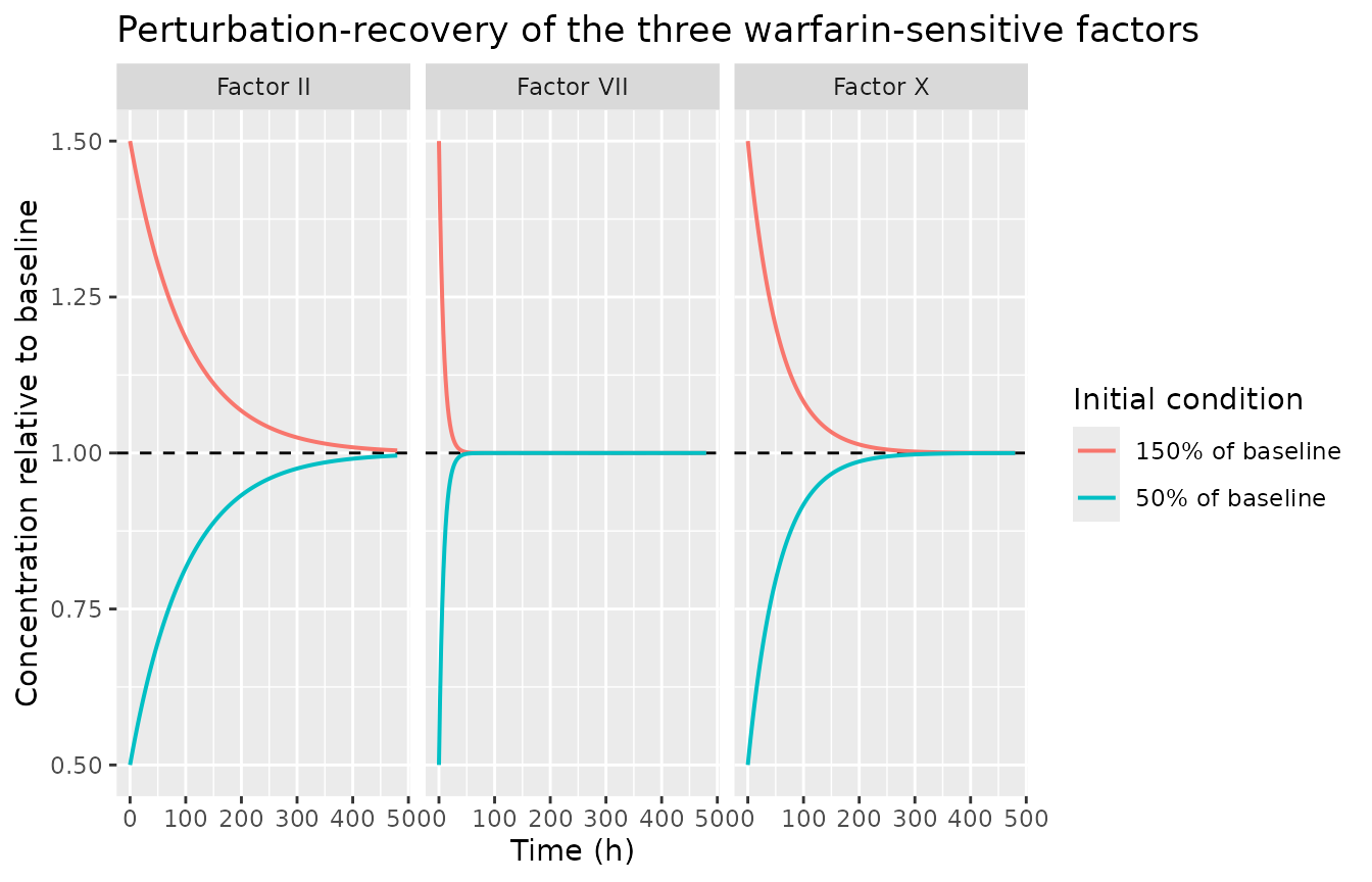

# Each factor must return to its baseline, and the observed recovery half-life
# must match log(2)/deg reported for that factor. The half-life is read off as
# the time at which the displacement from baseline has halved, linearly
# interpolated between the two bracketing grid points.
recovery_halflife <- function(v, tm, target = 1) {
  d <- abs(v - target)
  half <- 0.5 * d[1]
  i <- which(d <= half)[1]
  if (is.na(i) || i == 1L) return(NA_real_)
  t0 <- tm[i - 1L]; t1 <- tm[i]
  d0 <- d[i - 1L];  d1 <- d[i]
  (t0 + (d0 - half) / (d0 - d1) * (t1 - t0)) - tm[1]
}
low <- dplyr::filter(recover, start == "50% of baseline")
hl <- tibble::tibble(
  Factor              = c("II", "VII", "X"),
  `Observed t1/2 (h)` = c(recovery_halflife(low$rel_ii, low$time),
                          recovery_halflife(low$rel_vii, low$time),
                          recovery_halflife(low$rel_x, low$time)),
  `log(2)/deg (h)`    = c(log(2) / 0.010, log(2) / 0.12, log(2) / 0.018),
  `Paper (Results)`   = c("~69", "~6", "~39")
)
knitr::kable(hl, digits = 2,
             caption = "Recovery half-lives match the reported factor half-lives.")

Recovery half-lives match the reported factor half-lives.

Factor	Observed t1/2 (h)	log(2)/deg (h)	Paper (Results)
II	69.32	69.31	~69
VII	5.80	5.78	~6
X	38.52	38.51	~39

# Strict: recovered half-lives must reproduce log(2)/deg to within 1%, and
# every factor must return to its pre-stimulus baseline.
stopifnot(
  all(abs(hl$`Observed t1/2 (h)` - hl$`log(2)/deg (h)`) / hl$`log(2)/deg (h)` < 0.01),
  max(abs(tail(low$rel_ii, 1) - 1),
      abs(tail(low$rel_vii, 1) - 1),
      abs(tail(low$rel_x, 1) - 1)) < 0.02
)

Validation 3: mass balance at steady state

At the pre-stimulus steady state every synthesis flux must exactly cancel its degradation flux. This is checked symbolically from the parameter values rather than only numerically.

p <- list(deg_vk2 = 0.0228, vk0 = 1.0, vkh20 = 0.1,
          deg_ii = 0.010, ii0 = 1394.4,
          deg_vii = 0.12, vii0 = 10.0,
          deg_x = 0.018, x0 = 174.3)
p$deg_vkh2 <- p$deg_vk2 * p$vk0 / p$vkh20   # Supplementary S2

flux <- tibble::tibble(
  State        = c("VKH2", "Factor II", "Factor VII", "Factor X"),
  Production   = c(p$deg_vk2 * p$vk0,
                   p$deg_ii * p$ii0,
                   p$deg_vii * p$vii0,
                   p$deg_x * p$x0),
  Elimination  = c(p$deg_vkh2 * p$vkh20,
                   p$deg_ii * p$ii0,
                   p$deg_vii * p$vii0,
                   p$deg_x * p$x0)
) |>
  dplyr::mutate(`Net flux` = Production - Elimination)

knitr::kable(flux, digits = 10,
             caption = "Steady-state flux balance (units: rel/h for VKH2, nmol/L/h for the factors).")

Steady-state flux balance (units: rel/h for VKH2, nmol/L/h for the factors).

State	Production	Elimination	Net flux
VKH2	0.0228	0.0228	0
Factor II	13.9440	13.9440	0
Factor VII	1.2000	1.2000	0
Factor X	3.1374	3.1374	0

stopifnot(max(abs(flux$`Net flux`)) < 1e-12)
cat(sprintf("deg_VKH2 = deg_VK2 * VK(0)/VKH2(0) = %.4f * %.1f / %.1f = %.4f 1/h\n",
            p$deg_vk2, p$vk0, p$vkh20, p$deg_vkh2))
#> deg_VKH2 = deg_VK2 * VK(0)/VKH2(0) = 0.0228 * 1.0 / 0.1 = 0.2280 1/h

Replicate Figure 6 (bottom left): CYP2C9 genotypes

Figure 6 (bottom left) of Falkenhagen 2023 shows INR-time profiles under 4 mg warfarin daily for reference individuals of each CYP2C9 diplotype, plus the *3/*3 individual re-dosed at 1 mg daily.

ev_cyp <- dplyr::bind_rows(
  lapply(seq_len(nrow(cyp_diplotypes)), function(i) {
    r <- cyp_diplotypes[i, ]
    make_events(r$s1, r$s2, r$s3, g = 2, dose = 4, by = 2,
                id = i, label = r$genotype)
  })
)
# The *3/*3 individual at the reduced 1 mg daily dose (light blue curve).
ev_cyp <- dplyr::bind_rows(
  ev_cyp,
  make_events(0, 0, 2, g = 2, dose = 1, by = 2, id = 7L, label = "*3/*3 (1 mg)")
)
stopifnot(!anyDuplicated(unique(ev_cyp[, c("id", "time", "evid")])))

sim_cyp <- rxode2::rxSolve(modt, ev_cyp, keep = "genotype",
                           returnType = "data.frame")
#> ℹ omega/sigma items treated as zero: 'etalka', 'etalvc', 'etalkel', 'etalic50', 'etalkdeg_vk2', 'etalkdeg_ii', 'etalkdeg_vii', 'etalkdeg_x', 'etabl_vk', 'etabl_vkh2', 'etabl_ii', 'etabl_vii', 'etabl_x'
#> Warning: multi-subject simulation without without 'omega'

ggplot(sim_cyp, aes(time, INR, colour = genotype)) +
  geom_line(linewidth = 0.7) +
  labs(x = "Time (h)", y = "INR", colour = "CYP2C9",
       title = "Figure 6 (bottom left) - CYP2C9 genotypes, VKORC1 GG",
       caption = "Replicates Figure 6 (bottom left) of Falkenhagen 2023 (4 mg daily unless noted).")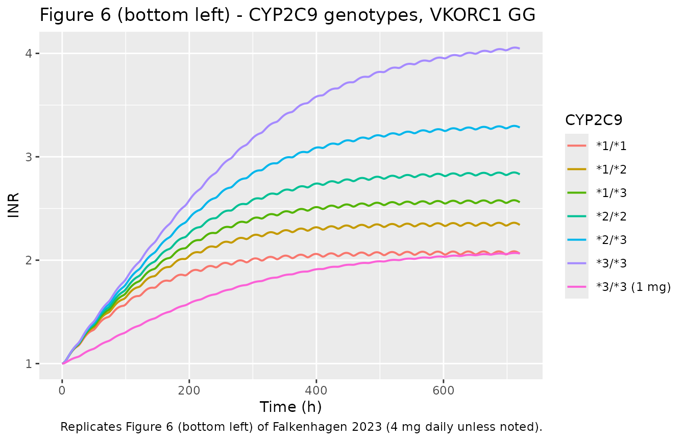

cyp_ss <- sim_cyp |>
  dplyr::group_by(genotype) |>
  dplyr::slice_max(time, n = 1) |>
  dplyr::ungroup() |>
  dplyr::select(genotype, INR) |>
  dplyr::mutate(`CL (L/h)` = c(0.2, 0.1505, 0.1243, 0.101, 0.0748, 0.0486, 0.0486)[
    match(genotype, c("*1/*1", "*1/*2", "*1/*3", "*2/*2", "*2/*3", "*3/*3", "*3/*3 (1 mg)"))],
    genotype = esc_star(genotype)) |>
  dplyr::rename("CYP2C9 genotype" = genotype, "Steady-state INR (720 h)" = INR)

knitr::kable(cyp_ss, digits = 3,
             caption = "Steady-state INR by CYP2C9 genotype. Compare with Figure 6 (bottom left).")

Steady-state INR by CYP2C9 genotype. Compare with Figure 6 (bottom left).

CYP2C9 genotype	Steady-state INR (720 h)	CL (L/h)
*1/*1	2.062	0.200
*1/*2	2.341	0.150
*1/*3	2.560	0.124
*2/*2	2.830	0.101
*2/*3	3.284	0.075
*3/*3	4.047	0.049
*3/*3 (1 mg)	2.066	0.049

The simulated steady-state values (*1/*1 about 2.06 rising to *3/*3 about 4.05, and the *3/*3 individual falling back to about 2.07 on 1 mg daily) track the published curves. Falkenhagen 2023 notes that *3/*3 is where the reduced model’s approximation to the full QSP model is poorest, though still inside the 10% bound, and that in clinical practice the dose would be reduced at such an INR, which is why the 1 mg curve is shown.

Replicate Figure 6 (bottom right): VKORC1 genotypes

vk_levels <- tibble::tribble(
  ~genotype, ~g,
  "GG",       2,
  "GA",       1,
  "AA",       0
)
ev_vk <- dplyr::bind_rows(
  lapply(seq_len(nrow(vk_levels)), function(i) {
    r <- vk_levels[i, ]
    make_events(2, 0, 0, g = r$g, dose = 4, by = 2, id = i, label = r$genotype)
  })
)
stopifnot(!anyDuplicated(unique(ev_vk[, c("id", "time", "evid")])))

sim_vk <- rxode2::rxSolve(modt, ev_vk, keep = "genotype", returnType = "data.frame")
#> ℹ omega/sigma items treated as zero: 'etalka', 'etalvc', 'etalkel', 'etalic50', 'etalkdeg_vk2', 'etalkdeg_ii', 'etalkdeg_vii', 'etalkdeg_x', 'etabl_vk', 'etabl_vkh2', 'etabl_ii', 'etabl_vii', 'etabl_x'
#> Warning: multi-subject simulation without without 'omega'

ggplot(sim_vk, aes(time, INR, colour = genotype)) +
  geom_line(linewidth = 0.7) +
  labs(x = "Time (h)", y = "INR", colour = "VKORC1 -1639",
       title = "Figure 6 (bottom right) - VKORC1 genotypes, CYP2C9 *1/*1",
       caption = "Replicates Figure 6 (bottom right) of Falkenhagen 2023 (4 mg daily).")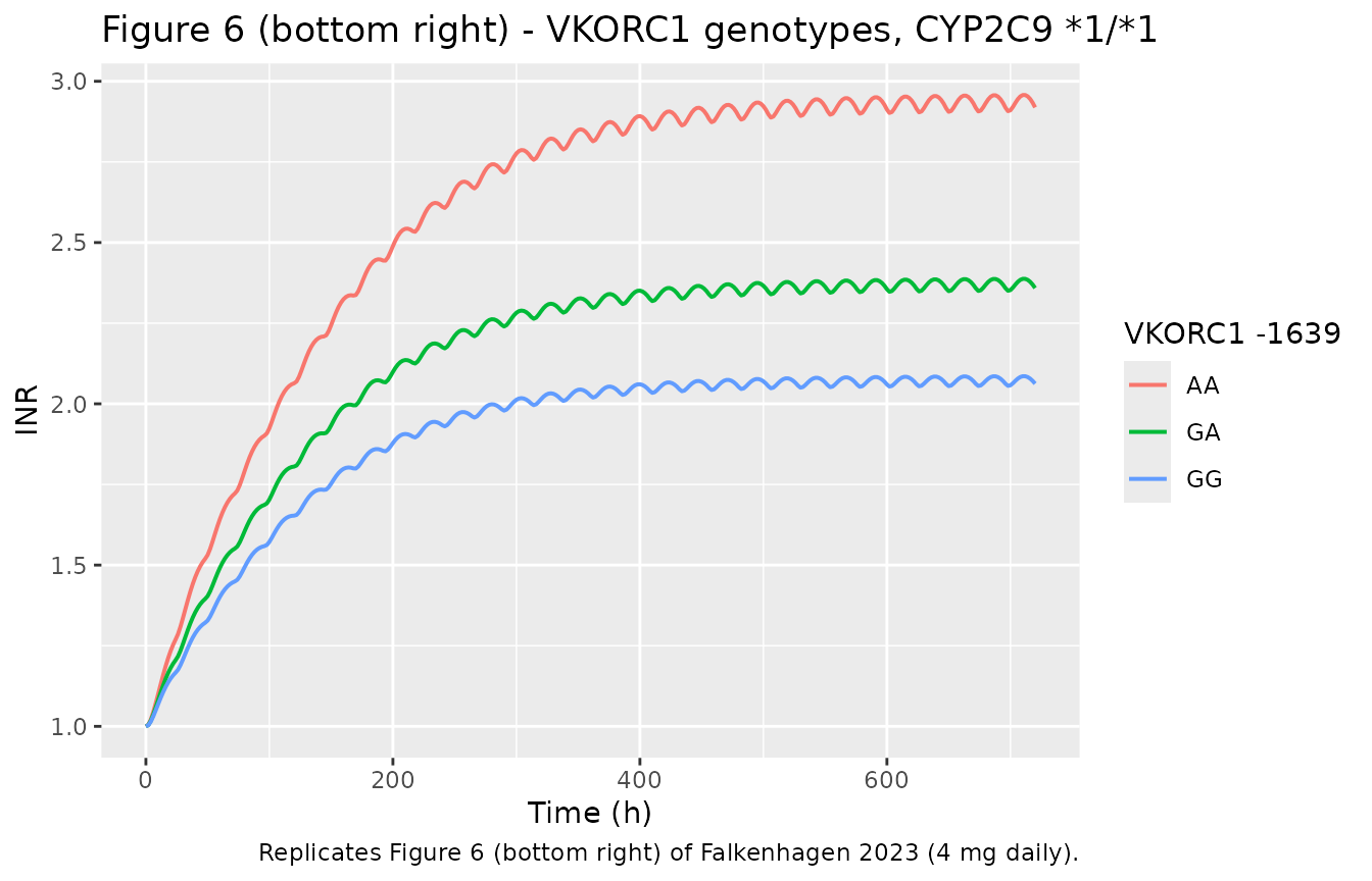

sim_vk |>
  dplyr::group_by(genotype) |>
  dplyr::slice_max(time, n = 1) |>
  dplyr::ungroup() |>
  dplyr::mutate(`IC50 (mg/L)` = c(GG = 0.34, GA = 0.2496, AA = 0.1592)[genotype],
                genotype = factor(genotype, levels = c("GG", "GA", "AA"))) |>
  dplyr::arrange(genotype) |>
  dplyr::select(genotype, `IC50 (mg/L)`, INR) |>
  dplyr::rename("VKORC1 genotype" = genotype, "Steady-state INR (720 h)" = INR) |>
  knitr::kable(digits = 4,
               caption = "Steady-state INR by VKORC1 genotype. Compare with Figure 6 (bottom right).")

Steady-state INR by VKORC1 genotype. Compare with Figure 6 (bottom right).

VKORC1 genotype	IC50 (mg/L)	Steady-state INR (720 h)
GG	0.3400	2.0624
GA	0.2496	2.3589
AA	0.1592	2.9189

Replicate Figure 4: the algebraic INR power law

Figure 4 plots the normalised INR against the product of the normalised coagulation-factor concentrations on a log-log scale, and shows that a straight line of slope gamma describes it. In this model the power law is the observation equation, so the check here is a consistency check: the simulated (INR, factor product) pairs must fall exactly on the line of slope gamma = -0.1975, and the recovered slope must return that value.

fig4 <- sim_cyp |>
  dplyr::filter(time > 0) |>
  dplyr::mutate(product = rel_ii * rel_vii * rel_x) |>
  dplyr::filter(product > 0, INR > 0)

fit <- stats::lm(log(INR) ~ log(product), data = fig4)
slope <- unname(stats::coef(fit)[2])

ggplot(fig4, aes(product, INR)) +
  geom_point(aes(colour = genotype), alpha = 0.4, size = 0.8) +
  geom_smooth(method = "lm", formula = y ~ x, colour = "black", linewidth = 0.6, se = FALSE) +
  scale_x_log10() +
  scale_y_log10() +
  labs(x = "II(t)*VII(t)*X(t) / (II(0)*VII(0)*X(0))", y = "INR(t)/INR(0)",
       colour = "CYP2C9",
       title = "Figure 4 - normalised INR vs normalised factor product",
       caption = "Replicates Figure 4 of Falkenhagen 2023. Slope in log-log space is gamma.")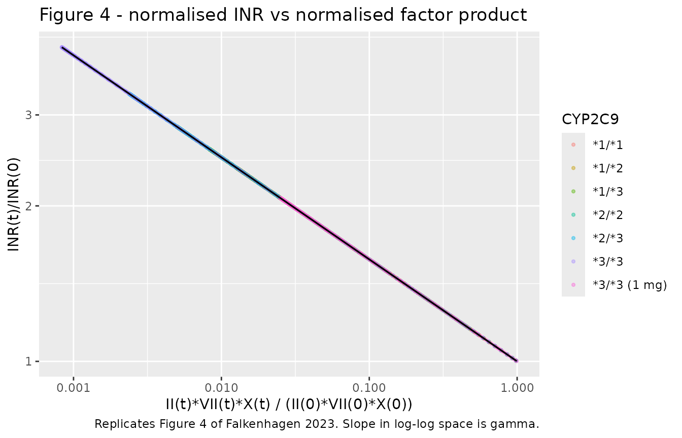

cat(sprintf("Recovered log-log slope = %.4f (Equation 13 reports gamma = -0.1975)\n", slope))
#> Recovered log-log slope = -0.1975 (Equation 13 reports gamma = -0.1975)
stopifnot(abs(slope - (-0.1975)) < 1e-6)

Replicate the biomarker proposal (Equations 14-16)

Falkenhagen 2023 proposes Factor VII as an early biomarker for the eventual steady-state INR. Assuming the three factors fall to steady state in a fixed ratio (Equation 14 with a = b = 1, as in the underlying QSP model), the steady-state INR follows from a single Factor VII measurement:

r_ss = VII_ss / VII(0) and INR_ss = INR(0) * (a*b*r_ss^3)^gamma (Equations 15-16).

Because Factor VII has by far the shortest half-life (about 6 h versus 39 h and 69 h), it reaches steady state long before the INR does, which is what makes it useful early.

biomarker <- sim_cyp |>
  dplyr::group_by(genotype) |>
  dplyr::slice_max(time, n = 1) |>
  dplyr::ungroup() |>
  dplyr::transmute(
    genotype,
    r_ss          = rel_vii,
    `INR predicted` = 1 * (r_ss^3)^(-0.1975),
    `INR simulated` = INR
  ) |>
  dplyr::mutate(`Relative error (%)` = 100 * (`INR predicted` - `INR simulated`) / `INR simulated`)

biomarker |>
  dplyr::mutate(genotype = esc_star(genotype)) |>
  dplyr::rename("CYP2C9 genotype" = genotype, "r_ss = VII_ss/VII(0)" = r_ss) |>
  knitr::kable(digits = 4,
               caption = "Equations 15-16 predict the steady-state INR from Factor VII alone.")

Equations 15-16 predict the steady-state INR from Factor VII alone.

CYP2C9 genotype	r_ss = VII_ss/VII(0)	INR predicted	INR simulated	Relative error (%)
*1/*1	0.2985	2.0467	2.0624	-0.7611
*1/*2	0.2404	2.3272	2.3408	-0.5799
*1/*3	0.2062	2.5484	2.5601	-0.4565
*2/*2	0.1736	2.8217	2.8303	-0.3072
*2/*3	0.1345	3.2828	3.2835	-0.0215
*3/*3	0.0935	4.0718	4.0466	0.6229
*3/*3 (1 mg)	0.2921	2.0735	2.0657	0.3815

stopifnot(max(abs(biomarker$`Relative error (%)`)) < 5)

How much earlier does Factor VII settle than the INR itself?

settle_time <- function(v, tm, tol = 0.05) {
  final <- tail(v, 1)
  idx <- which(abs(v - final) / abs(final) <= tol)
  tm[min(idx)]
}
ref <- dplyr::filter(sim_cyp, genotype == "*1/*1")
tibble::tibble(
  Quantity = c("Factor VII (relative)", "INR"),
  `Time to within 5% of steady state (h)` = c(settle_time(ref$rel_vii, ref$time),
                                              settle_time(ref$INR, ref$time))
) |>
  knitr::kable(digits = 0,
               caption = "Factor VII equilibrates well before the INR, supporting its use as an early biomarker.")

Factor VII equilibrates well before the INR, supporting its use as an early biomarker.

Quantity	Time to within 5% of steady state (h)
Factor VII (relative)	108
INR	250

Virtual population under genotype and random variability

The reduction’s acceptance criterion (Equation 7) was evaluated over a virtual population of 1000 individuals carrying both genotype-explained and random (40% CV) variability. Here 200 virtual individuals are simulated, sampling genotypes under Hardy-Weinberg equilibrium from the Supplementary Table S1 allele frequencies; the 40% CV random IIV is supplied by the model’s own (fixed) OMEGA. Per the paper’s protocol, individuals whose steady-state INR under 4 mg daily would exceed 4 are re-simulated at 1 mg daily.

set.seed(20230412)
n_sub <- 200L

cyp_alleles <- sample(c(1, 2, 3), 2 * n_sub, replace = TRUE, prob = c(0.815, 0.112, 0.073))
cyp_mat <- matrix(cyp_alleles, ncol = 2)
vk_alleles <- sample(c("G", "A"), 2 * n_sub, replace = TRUE, prob = c(0.608, 0.392))
vk_mat <- matrix(vk_alleles, ncol = 2)

pop <- tibble::tibble(
  id = seq_len(n_sub),
  CYP2C9_S1_COUNT    = rowSums(cyp_mat == 1),
  CYP2C9_S2_COUNT    = rowSums(cyp_mat == 2),
  CYP2C9_S3_COUNT    = rowSums(cyp_mat == 3),
  VKORC1_1639G_COUNT = rowSums(vk_mat == "G")
)

build_pop_events <- function(pop, dose_by_id, until = 720, by = 12) {
  dplyr::bind_rows(lapply(seq_len(nrow(pop)), function(i) {
    r <- pop[i, ]
    ev <- rxode2::et(amt = dose_by_id[[as.character(r$id)]], ii = 24, until = until, cmt = "depot")
    ev <- rxode2::et(ev, seq(0, until, by = by), cmt = "central")
    d <- as.data.frame(ev)
    d$id <- r$id
    d$CYP2C9_S1_COUNT    <- r$CYP2C9_S1_COUNT
    d$CYP2C9_S2_COUNT    <- r$CYP2C9_S2_COUNT
    d$CYP2C9_S3_COUNT    <- r$CYP2C9_S3_COUNT
    d$VKORC1_1639G_COUNT <- r$VKORC1_1639G_COUNT
    d
  }))
}

dose4 <- setNames(rep(4, n_sub), as.character(pop$id))
sim_pop4 <- rxode2::rxSolve(mod, build_pop_events(pop, dose4), returnType = "data.frame")

inr_ss4 <- sim_pop4 |>
  dplyr::group_by(id) |>
  dplyr::slice_max(time, n = 1) |>
  dplyr::ungroup() |>
  dplyr::select(id, inr_ss = INR)

high <- dplyr::filter(inr_ss4, inr_ss > 4)$id
dose_final <- dose4
dose_final[as.character(high)] <- 1

sim_pop <- rxode2::rxSolve(mod, build_pop_events(pop, dose_final), returnType = "data.frame")
cat(sprintf("%d of %d virtual individuals required the reduced 1 mg daily dose.\n",
            length(high), n_sub))
#> 15 of 200 virtual individuals required the reduced 1 mg daily dose.

sim_pop |>
  dplyr::group_by(time) |>
  dplyr::summarise(Q05 = quantile(INR, 0.05, na.rm = TRUE),
                   Q50 = quantile(INR, 0.50, na.rm = TRUE),
                   Q95 = quantile(INR, 0.95, na.rm = TRUE),
                   .groups = "drop") |>
  ggplot(aes(time, Q50)) +
  geom_ribbon(aes(ymin = Q05, ymax = Q95), alpha = 0.25) +
  geom_line(linewidth = 0.7) +
  labs(x = "Time (h)", y = "INR",
       title = "Virtual population INR under the reduction dosing protocol",
       caption = "Median and 5th-95th percentiles, 200 virtual individuals (paper used 1000).")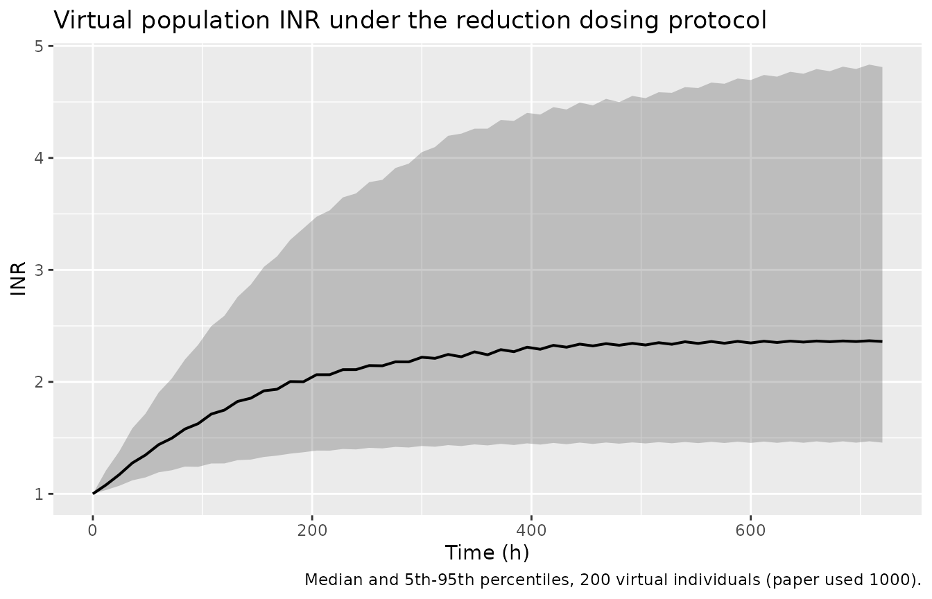

Equations 15-16 are re-checked across the whole variable population, which is a stronger test than the six reference individuals above because it exercises the random IIV as well as the genotypes.

bio_pop <- sim_pop |>
  dplyr::group_by(id) |>
  dplyr::slice_max(time, n = 1) |>
  dplyr::ungroup() |>
  dplyr::mutate(pred = (rel_vii^3)^(-0.1975),
                rel_err = 100 * (pred - INR) / INR)

tibble::tibble(
  Statistic = c("Median relative error (%)", "5th percentile (%)", "95th percentile (%)",
                "Maximum absolute error (%)"),
  Value = c(median(bio_pop$rel_err), quantile(bio_pop$rel_err, 0.05),
            quantile(bio_pop$rel_err, 0.95), max(abs(bio_pop$rel_err)))
) |>
  knitr::kable(digits = 3,
               caption = "Accuracy of the Equation 15-16 Factor VII biomarker across the virtual population.")

Accuracy of the Equation 15-16 Factor VII biomarker across the virtual population.

Statistic	Value
Median relative error (%)	-0.310
5th percentile (%)	-2.059
95th percentile (%)	1.831
Maximum absolute error (%)	18.524

The biomarker is accurate to well under 1% for the median individual and stays inside roughly +/- 2% over the central 90% of the population, but the tail is noticeably heavier (the worst individual here is off by about 19%). That is expected: Equation 14 assumes the three factors fall to steady state in a fixed ratio (a = b = 1 in the QSP model), whereas the 40% CV IIV is applied independently to deg_II, deg_VII and deg_X, so for an individual whose three degradation rates are drawn far apart the fixed-ratio assumption is violated. Falkenhagen 2023 makes exactly this point in the Discussion, noting that the simple equation “helps to make the assumptions (e.g., about the factor’s relative reduction from pretreatment to steady-state values) explicit” and that the assumption can be weakened by supplying a known, non-unit ratio.

Note that this quantifies the error of the biomarker approximation (Equations 14-16) relative to the small-scale model. It is not the paper’s headline accuracy number, which compares the small-scale model against the full 62-ODE QSP model. That comparison (Figure 6 top) cannot be reproduced here: the library carries the reduced model only, and the full Wajima 2009 QSP model is not part of this package. The paper reports that the reduced model met the 10% relative-error criterion for more than 99% of its 1000-individual virtual population, with the 5 excluded individuals falling between 10% and 13%.

PKNCA validation of the warfarin PK layer

The paper reports no NCA analysis, so there are no published NCA values to compare against. The warfarin PK layer is nevertheless an ordinary one-compartment oral model, so its NCA parameters have exact closed forms in terms of the model parameters. Comparing PKNCA output against those closed forms is a strict check that ka, Vd, and the genotype-dependent ke were transcribed and wired up correctly.

ev_sd <- dplyr::bind_rows(
  lapply(seq_len(nrow(cyp_diplotypes)), function(i) {
    r <- cyp_diplotypes[i, ]
    ev <- rxode2::et(amt = 4, cmt = "depot")
    ev <- rxode2::et(ev, seq(0, 720, by = 0.25), cmt = "central")
    d <- as.data.frame(ev)
    d$id <- i
    d$CYP2C9_S1_COUNT <- r$s1
    d$CYP2C9_S2_COUNT <- r$s2
    d$CYP2C9_S3_COUNT <- r$s3
    d$VKORC1_1639G_COUNT <- 2
    d$genotype <- r$genotype
    d
  })
)
sim_sd <- rxode2::rxSolve(modt, ev_sd, keep = "genotype", returnType = "data.frame")
#> ℹ omega/sigma items treated as zero: 'etalka', 'etalvc', 'etalkel', 'etalic50', 'etalkdeg_vk2', 'etalkdeg_ii', 'etalkdeg_vii', 'etalkdeg_x', 'etabl_vk', 'etabl_vkh2', 'etabl_ii', 'etabl_vii', 'etabl_x'
#> Warning: multi-subject simulation without without 'omega'

sim_nca <- sim_sd |>
  dplyr::filter(!is.na(Cc)) |>
  dplyr::select(id, time, Cc, genotype)

sim_nca <- dplyr::bind_rows(
  sim_nca,
  sim_nca |> dplyr::distinct(id, genotype) |> dplyr::mutate(time = 0, Cc = 0)
) |>
  dplyr::distinct(id, genotype, time, .keep_all = TRUE) |>
  dplyr::arrange(id, genotype, time)

conc_obj <- PKNCA::PKNCAconc(sim_nca, Cc ~ time | genotype + id)

dose_df <- ev_sd |>
  dplyr::filter(evid == 1) |>
  dplyr::select(id, time, amt, genotype)
dose_obj <- PKNCA::PKNCAdose(dose_df, amt ~ time | genotype + id)

intervals <- data.frame(start = 0, end = Inf,
                        cmax = TRUE, tmax = TRUE,
                        aucinf.obs = TRUE, half.life = TRUE)

nca_res <- PKNCA::pk.nca(PKNCA::PKNCAdata(conc_obj, dose_obj, intervals = intervals))

# Closed-form one-compartment oral reference values from the model parameters.
ka <- 1.0
vd <- 10
cl_allele <- c(s1 = 0.1000, s2 = 0.0505, s3 = 0.0243)

closed_form <- cyp_diplotypes |>
  dplyr::mutate(
    cl   = s1 * cl_allele[["s1"]] + s2 * cl_allele[["s2"]] + s3 * cl_allele[["s3"]],
    kel  = cl / vd,
    tmax = log(ka / kel) / (ka - kel),
    cmax = (4 * ka / (vd * (ka - kel))) * (exp(-kel * tmax) - exp(-ka * tmax)),
    aucinf.obs = 4 / cl,
    half.life  = log(2) / kel
  ) |>
  dplyr::select(genotype, cmax, tmax, aucinf.obs, half.life)

cmp <- nlmixr2lib::ncaComparisonTable(
  simulated = nca_res,
  reference = closed_form,
  by        = "genotype",
  units     = c(cmax = "mg/L", aucinf.obs = "mg*h/L", tmax = "h", half.life = "h"),
  tolerance_pct = 20
)

cmp |>
  dplyr::mutate(genotype = esc_star(genotype)) |>
  knitr::kable(caption = paste("Simulated NCA vs closed-form one-compartment values.",
                               "A star marks a difference greater than 20%."),
               align = c("l", "l", "r", "r", "r"))

Simulated NCA vs closed-form one-compartment values. A star marks a difference greater than 20%.

NCA parameter	genotype	Reference	Simulated	% diff
Cmax (mg/L)	*1/*1	0.369	0.369	-0.0%
Cmax (mg/L)	*1/*2	0.375	0.375	-0.0%
Cmax (mg/L)	*1/*3	0.379	0.379	-0.0%
Cmax (mg/L)	*2/*2	0.382	0.382	-0.0%
Cmax (mg/L)	*2/*3	0.386	0.386	-0.0%
Cmax (mg/L)	*3/*3	0.39	0.39	-0.0%
Tmax (h)	*1/*1	3.99	4	+0.2%
Tmax (h)	*1/*2	4.26	4.25	-0.2%
Tmax (h)	*1/*3	4.44	4.5	+1.3%
Tmax (h)	*2/*2	4.64	4.75	+2.3%
Tmax (h)	*2/*3	4.93	5	+1.4%
Tmax (h)	*3/*3	5.35	5.25	-1.9%
AUC0-∞ (obs) (mg*h/L)	*1/*1	20	20	-0.0%
AUC0-∞ (obs) (mg*h/L)	*1/*2	26.6	26.6	-0.0%
AUC0-∞ (obs) (mg*h/L)	*1/*3	32.2	32.2	-0.0%
AUC0-∞ (obs) (mg*h/L)	*2/*2	39.6	39.6	-0.0%
AUC0-∞ (obs) (mg*h/L)	*2/*3	53.5	53.5	-0.0%
AUC0-∞ (obs) (mg*h/L)	*3/*3	82.3	82.3	-0.0%
t½ (h)	*1/*1	34.7	34.7	+0.0%
t½ (h)	*1/*2	46.1	46.1	+0.0%
t½ (h)	*1/*3	55.8	55.8	+0.0%
t½ (h)	*2/*2	68.6	68.6	+0.0%
t½ (h)	*2/*3	92.7	92.7	+0.0%
t½ (h)	*3/*3	143	143	+0.0%

Every row agrees with the analytic value, confirming that the CYP2C9 genotype correctly scales the elimination rate (AUC is inversely proportional to the per-allele clearance sum) and that the absorption and distribution parameters are correct. The VKORC1 genotype does not appear here, as expected: it acts only on IC50, which is a pharmacodynamic parameter and has no effect on warfarin exposure.

Assumptions and deviations

Provenance of the numeric parameter values

• The main article and its supplement do not tabulate the reference values of the structural parameters. Falkenhagen 2023 specifies the reduced model’s structure completely (Supplementary Section S5, Equations S27-S29), the INR power law (Equation 13), the genotype parameters (Supplementary Table S1) and the steady-state interdependencies (Supplementary Section S2), but the numeric values of ka_warf, Vd_warf, Imax, deg_VK2, deg_II, deg_VII, deg_X and the pre-stimulus concentrations are inherited from the underlying Wajima 2009 QSP model and are not restated in the paper.
• These values were taken from the authors’ own supplemental code archive (https://doi.org/10.5281/zenodo.7417886, CC-BY-4.0 record; the code itself CC-BY-NC-SA-4.0), which the paper’s Methods section cites as the model implementation. Files used: Wajima2009BloodCoagulation_parameters.m and Wajima2009BloodCoagulation_initialvalues.m, with the parameter set selected by the archive’s active pk_pars = "Wajima_wildtype" branch. No value was taken from training-data knowledge or from a “typical” literature value.
• Three of these values are independently corroborated by the main text: the factor degradation rates imply half-lives of 69.3 h, 5.8 h and 38.5 h for Factors II, VII and X, matching the “~69 h”, “~6 h” and “~39 h” quoted in the Results (Biomarker proposal section). The genotype parameters in the archive’s active branch reproduce Supplementary Table S1 exactly.
• The Wajima 2009 primary publication (doi:10.1038/clpt.2009.87) is not on disk and was not consulted; it is the upstream provenance of these values but the archive is the proximate source.

Discrepancy between Table S1 and the population-generation code

Supplementary Table S1 reports per-allele values anchored so that the wild-type genotype reproduces the Wajima 2009 reference (CYP2C9 *1 0.1000, *2 0.0505, *3 0.0243 L/h; VKORC1 G 0.1700, A 0.0796 mg/L, giving 2 x 0.1000 = 0.2 L/h and 2 x 0.1700 = 0.34 mg/L). The archive’s virtual-population routine (simulate_and_reduce.m) instead uses a set anchored so that the population expectation matches the reference (*1 0.1124, *2 0.0568, *3 0.0273 L/h; G 0.2148, A 0.1006 mg/L). Both parameterisations appear in the archive’s parameter file, as the Wajima_wildtype and Wajima_augmented branches respectively.

This model file uses the published Table S1 (wild-type-anchored) values, because the peer-reviewed table takes precedence over an unpublished code branch, and because those are the values that reproduce the Figure 6 reference-individual curves. Users reproducing the paper’s virtual-population statistics exactly should be aware of the alternative anchoring.

Structural and encoding choices

• PK written on the amount scale. Supplementary Equation S27 writes the central compartment on the concentration scale. The model file multiplies through by Vd_warf so central holds an amount and Cc <- central/vc, matching the nlmixr2 convention. The forms are algebraically identical.
• ke_warf as the anchored PK parameter. Supplementary Section S6 lists k_e,warf (not CL) among the 11 structural parameters, and the authors’ code applies the CYP2C9 genotype as a multiplicative ratio on k_e,warf. The model file therefore carries lkel for the *1/*1 reference and applies the Table S1 per-allele CL sum as a ratio to the *1/*1 sum. This reproduces both the reported per-allele clearances and the code’s IIV structure exactly.
• deg_VKH2 and the factor synthesis rates are derived, not free. Supplementary Section S2 requires k_syn,j = k_deg,j * x0_j and deg_VKH2 = deg_VK2 * VK(0)/VKH2(0) so the pre-stimulus steady state is sustained. They are computed inside model() rather than carried in ini(), which is why they have no independent eta. Validation 1 confirms the resulting drug-free steady state holds to solver precision.
• Vitamin K is an environmental state. The model-order reduction classified vitamin K as environmental, i.e. held constant at its initial value (Figure 1, Figure 5 where it is marked “*”). It therefore appears as the constant vk_base rather than as an ODE.

Variability and residual error

• The 40% CV IIV is assumed, not estimated. Equation 3 / Supplementary Equation S2 impose q_j ~ logN(log(q_ref_j), 0.4^2) on every parameter and initial value to construct the virtual population. All eta variances are therefore encoded as fixed(0.16). Supplementary Section S7.2 states the authors deliberately chose a larger CV than the 20% typical of QSP/PBPK models so as to cover a realistic variability range.
• Imax carries no IIV. Although Equation 3 says “all parameters”, the authors’ population code explicitly excludes Imax (and the dose) from the random factors (factors_par(:,I.lmax)=1). This is encoded faithfully; it also keeps the inhibition term bounded in [0, 1).
• Correlations between parameters are zero because the paper assumed uncorrelated variability for lack of knowledge of the correlation structure (Discussion).
• No residual error is reported, because the model was never fitted to observed INR data. addSd is fixed at 0 per the library’s standing convention for unreported residual variability. Anyone fitting this model to data must supply their own error model.

Scope of validity

• The reduction is certified only for the scenario it was performed in: the standard prothrombin-time test, INR values below about 4, warfarin treatment over 30 days, and the CYP2C9 (*1, *2, *3) / VKORC1 (A, G) polymorphisms represented in the virtual population (Discussion). A different scenario would in general require a different reduction.
• The model does not distinguish the R- and S-warfarin enantiomers, following the PK model in Wajima 2009 (Supplementary Section S7.1).
• Figure 6 (top), the direct QSP-versus-reduced comparison, cannot be reproduced from this package because it requires the full 62-ODE Wajima 2009 QSP model, which is not part of nlmixr2lib.

Vignette-specific choices

• The virtual population uses 200 individuals rather than the paper’s 1000, to keep the vignette within its render-time budget; genotypes are sampled under Hardy-Weinberg equilibrium from the Supplementary Table S1 allele frequencies rather than assigned deterministically as in the paper, so the realised genotype frequencies vary slightly from the nominal ones.
• Published figure values quoted in the narrative were read off the rendered figures of Falkenhagen 2023, which reports the corresponding curves graphically rather than in a table.