Melanoma tumor size dynamics under pembrolizumab (Chatterjee 2017) • nlmixr2lib

The paper and the two models

Chatterjee 2017 reports two longitudinal tumor-size models for pembrolizumab in advanced melanoma, built at two different points on the programme’s regulatory path, and this library packages both:

Model file	Approach	Dataset	Final parameters
`Chatterjee_2017_pembrolizumab_mixture`	four-class latent mixture, plus a second-stage multinomial regression on the class logits	KEYNOTE-001 only, N = 364, October 2013 cutoff	main-article Table 2 and supplementary Table 2B
`Chatterjee_2017_pembrolizumab_consolidated`	one continuous structure with between-subject variability in three parameters	pooled KEYNOTE-001, -002 and -006, N = 1,366, April 2015 cutoff	supplementary Table 4C

Both are pharmacodynamic (tumor growth inhibition) models, not PK models. The observable TS is the RECIST version 1.1 sum of the longest diameters of target lesions, in mm. There is no PKNCA section in this vignette: neither model has a concentration output or a dosing event, so non-compartmental analysis has nothing to act on. Exposure enters both models only through the per-subject covariate AUC_PEMBRO (AUCss-6weeks), which the source analysis obtained from a separate population-PK analysis of the same programme – published as Ahamadi 2017 and packaged in this library as Ahamadi_2017_pembrolizumab. The validation below is therefore structural (closed-form and covariate-effect identities) plus a reproduction of the paper’s own simulated response rates.

mix <- rxode2::rxode2(readModelDb("Chatterjee_2017_pembrolizumab_mixture"))
#> ℹ Four-class mixture tumor-size model for pembrolizumab in advanced melanoma (Chatterjee 2017; KEYNOTE-001, n = 364). Observable `TS` is the RECIST 1.1 sum of longest diameters in mm, TS(t) = BASEL1 * exp((KL - KD) * t) + BASEL2. Assign each subject a latent class with the binary covariates MIX_MONO_SLOW / MIX_BIPHASIC / MIX_MONO_FAST (all three 0 = the reference 'escape' class); the file also returns the paper's second-stage multinomial class probabilities prob_escape / prob_monophasic_slow / prob_biphasic / prob_monophasic_fast for that assignment. Required covariates: MIX_MONO_SLOW, MIX_BIPHASIC, MIX_MONO_FAST, NTARGET, WHO_PS, TUM_SLD, NNODAL, AUC_PEMBRO. No PK input: supply exposure per subject as AUC_PEMBRO (mg*day/L), which the source computed as dose/CL from the companion popPK model packaged here as Ahamadi_2017_pembrolizumab. Exposure affects only the class probabilities, and the paper's conclusion is that response is flat across 2-10 mg/kg.
#> ℹ parameter labels from comments will be replaced by 'label()'
con <- rxode2::rxode2(readModelDb("Chatterjee_2017_pembrolizumab_consolidated"))
#> ℹ Consolidated exposure-response tumor-size model for pembrolizumab in advanced melanoma (Chatterjee 2017; pooled KEYNOTE-001/-002/-006, N = 1,366). Observable `TS` is the RECIST 1.1 sum of longest diameters in mm. Bi-exponential: a treatment-accessible fraction f decaying at kdeath after a per-subject delay plus a resistant fraction (1 - f) growing at kgrowth, both initialised from the observed baseline covariate TUM_SLD. No PK input -- supply exposure per subject as AUC_PEMBRO (mg*day/L), which the source computed from the companion popPK model packaged here as Ahamadi_2017_pembrolizumab. Required covariates: TUM_SLD, AUC_PEMBRO, PRIOR_IPI, PDL1_TUM_POS, PDL1_TUM_MISSING, TUM_BRAF_MUT, T_SCAN_TO_DOSE. Note the reference categories: PD-L1-POSITIVE, BRAF wild type and IPI-naive. Neither exposure exponent on kdeath (0.131 IPI-naive, 0.100 IPI-experienced) is statistically significant (P = 0.20 and P = 0.25); the paper's conclusion is that response is flat across the fivefold 2-10 mg/kg dose range.

Citation: Chatterjee MS, Elassaiss-Schaap J, Lindauer A, Turner DC, Sostelly A, Freshwater T, Mayawala K, Ahamadi M, Stone JA, de Greef R, Kondic AG, de Alwis DP. Population pharmacokinetic/pharmacodynamic modeling of tumor size dynamics in pembrolizumab-treated advanced melanoma. CPT Pharmacometrics Syst Pharmacol. 2017;6(1):29-39. doi:10.1002/psp4.12140. PMID: 27896901. PMCID: PMC5270297. Structural equation from the main-article Methods (‘Consolidated exposure-response tumor size model’); all final parameter values from supplementary Table 4C (‘Parameter and uncertainty estimates of the final covariate-containing tumor model’); covariate functional forms, reference categories and centering constants from the supplementary NONMEM control stream (‘Final tumor size model, consolidated modeling approach’) and the Supplementary Methods (‘Consolidated Model Covariate Parameterization’).
Article: CPT Pharmacometrics Syst Pharmacol. 2017;6(1):29-39
Supplement: Supplementary Methods, Figures 1-4 and Tables 1-5, plus the three final NONMEM control streams, available open access with the article (PMC5270297).

The supplementary control streams are load-bearing for this extraction. They are the only place the source states the per-class structural switches, the covariate functional forms, the centering constants (98.15 mm, 80.75 mm, 6000 and 7079 mg*day/L, 3 target lesions) and the residual-error form. Note that their $THETA, $OMEGA and $SIGMA blocks carry initial estimates, not final ones – every value in both model files comes from the published parameter tables instead.

Population

pop <- con$meta$population
tibble::tibble(
  Field = c("Species", "Subjects", "Studies", "Age", "Weight", "Female", "Disease", "Doses"),
  Value = c(
    pop$species, format(pop$n_subjects, big.mark = ","), as.character(pop$n_studies),
    paste0(pop$age_median, " (", pop$age_range, ")"),
    paste0(pop$weight_median, " (", pop$weight_range, ")"),
    paste0(pop$sex_female_pct, "%"), pop$disease_state, pop$dose_range
  )
) |>
  knitr::kable(caption = "Consolidated-model population (Chatterjee 2017 Table 1, supplementary Tables 5A and 5B).")

Consolidated-model population (Chatterjee 2017 Table 1, supplementary Tables 5A and 5B).
Field	Value
Species	human (adults with unresectable or metastatic melanoma)
Subjects	1,366
Studies	3
Age	62.00 years (15.00-94.00 years (supplementary Table 5B))
Weight	79.30 kg (36.20-209.50 kg)
Female	39.02%
Disease	advanced (unresectable stage III or stage IV) melanoma; 620 of 1366 (45.39%) previously treated with or refractory to ipilimumab
Doses	pembrolizumab 2 mg/kg IV Q3W, 10 mg/kg IV Q3W, or 10 mg/kg IV Q2W (not a model input; enters only through AUC_PEMBRO)

The mixture-model population is the KEYNOTE-001 subset only: 364 patients, 51 at 10 mg/kg Q2W, 167 at 10 mg/kg Q3W and 146 at 2 mg/kg Q3W, of whom 168 were ipilimumab-naive (main-article Methods).

The imbalance that drives the consolidated model’s most unusual feature – two separate exposure-response slopes – is in Table 1: only 8.58% of the ipilimumab-naive patients were in the 2 mg/kg Q3W group against 38.23% of the ipilimumab-experienced patients.

Source trace

Every ini() value in both files, with its source location.

tibble::tribble(
  ~Model, ~Parameter, ~Value, ~Source,
  "mixture", "lkgrowth", "2.76e-3 /day", "Table 2, KL (log-estimated, back-transformed)",
  "mixture", "lkdeath", "3.57e-3 /day", "Table 2, KD (log-estimated, back-transformed)",
  "mixture", "lrbase_shallow", "56.3 mm", "Table 2, BASEL1",
  "mixture", "lrbase_deep", "25.1 mm", "Table 2, BASEL2",
  "mixture", "e_ntarget_lrbase_shallow", "0.654", "Table 2, BASEL1~NTARGET; power form and reference 3.00 from the control stream",
  "mixture", "e_ecog1_lrbase_shallow", "0.344", "Table 2, BASEL1~BECOGN; two-category form from the control stream",
  "mixture", "e_mix_escape_lrbase_shallow", "2", "Table 2, BASEL Rel. Diff.; applies to the escape class (supplementary Table 1)",
  "mixture", "e_mix_fast_kdeath", "4.17", "Table 2, KD Rel. Diff.; applies to the biphasic and monophasic-fast classes (supplementary Table 1)",
  "mixture", "lgt_mono_slow / lgt_biphasic / lgt_mono_fast", "0.325 / -0.0834 / -1.64", "supplementary Table 2B, BL2 / BL3 / BL4",
  "mixture", "e_auc_lgt", "5.61e-5 per mg*day/L", "supplementary Table 2B, beta_AUC2; centering 6000 from the control stream",
  "mixture", "e_nnodal_lgt", "0.112", "supplementary Table 2B, beta_NNODAL (uncentred)",
  "mixture", "e_tumsld_lgt", "-6.72e-3 per mm", "supplementary Table 2B, beta_BASE; centering 98.15 mm from the control stream",
  "mixture", "etalkdeath", "34% CV", "Table 2, IIV KD",
  "mixture", "etalrbase_shallow / etalrbase_deep", "79.6% / 225% CV, corr 0.863", "Table 2, IIV BL1, IIV BL2, Corr BL1~BL2",
  "mixture", "etalrv", "26.1% CV", "Table 2, ETA_EPS",
  "mixture", "(no eta on lkgrowth)", "fixed to zero", "control stream, $OMEGA 0 FIX ; IIV_KL",
  "mixture", "propSd / addSd", "10.3% / 3.29 mm", "Table 2, residual error; combined log-scale form from the control stream",
  "consolidated", "lkgrowth", "5.12e-4 /day", "supplementary Table 4C, kgrowth",
  "consolidated", "lkdeath", "6.09e-3 /day", "supplementary Table 4C, kdeath",
  "consolidated", "logitfresp", "f = 0.696", "supplementary Table 4C, f (natural scale; logit transform per Supplementary Methods)",
  "consolidated", "e_auc_kdeath_ipinaive", "0.131", "supplementary Table 4C, IPI naive AUC exponent",
  "consolidated", "e_auc_kdeath_ipiexp", "0.1", "supplementary Table 4C, IPI experienced AUC exponent",
  "consolidated", "e_pdl1_missing_kdeath", "-0.21", "supplementary Table 4C, PD-L1_1 on kdeath",
  "consolidated", "e_pdl1_neg_kdeath", "-0.614", "supplementary Table 4C, PD-L1_2 on kdeath",
  "consolidated", "e_braf_mut_kgrowth", "0.702", "supplementary Table 4C, BRAF_1 on kgrowth",
  "consolidated", "e_tumsld_kdeath", "-0.186", "supplementary Table 4C, baseline tumor size on kdeath (power, centered 80.75 mm)",
  "consolidated", "e_tumsld_fresp", "-0.00541 per mm", "supplementary Table 4C, Baseline Tumor Size on f (linear on logit, centered 80.75 mm)",
  "consolidated", "e_ipi_fresp", "-0.964", "supplementary Table 4C, IPIN_1 on f",
  "consolidated", "IIV block(3)", "1.64 / -1.24 / 1.39 / -1.54 / 1.07 / 5.53", "supplementary Table 4C, interindividual variability matrix",
  "consolidated", "expSd", "sqrt(0.0389)", "supplementary Table 4C, exponential residual (a variance)"
) |>
  knitr::kable(caption = "Source trace for both model files.")

Source trace for both model files.
Model	Parameter	Value	Source
mixture	lkgrowth	2.76e-3 /day	Table 2, KL (log-estimated, back-transformed)
mixture	lkdeath	3.57e-3 /day	Table 2, KD (log-estimated, back-transformed)
mixture	lrbase_shallow	56.3 mm	Table 2, BASEL1
mixture	lrbase_deep	25.1 mm	Table 2, BASEL2
mixture	e_ntarget_lrbase_shallow	0.654	Table 2, BASEL1~NTARGET; power form and reference 3.00 from the control stream
mixture	e_ecog1_lrbase_shallow	0.344	Table 2, BASEL1~BECOGN; two-category form from the control stream
mixture	e_mix_escape_lrbase_shallow	2	Table 2, BASEL Rel. Diff.; applies to the escape class (supplementary Table 1)
mixture	e_mix_fast_kdeath	4.17	Table 2, KD Rel. Diff.; applies to the biphasic and monophasic-fast classes (supplementary Table 1)
mixture	lgt_mono_slow / lgt_biphasic / lgt_mono_fast	0.325 / -0.0834 / -1.64	supplementary Table 2B, BL2 / BL3 / BL4
mixture	e_auc_lgt	5.61e-5 per mg*day/L	supplementary Table 2B, beta_AUC2; centering 6000 from the control stream
mixture	e_nnodal_lgt	0.112	supplementary Table 2B, beta_NNODAL (uncentred)
mixture	e_tumsld_lgt	-6.72e-3 per mm	supplementary Table 2B, beta_BASE; centering 98.15 mm from the control stream
mixture	etalkdeath	34% CV	Table 2, IIV KD
mixture	etalrbase_shallow / etalrbase_deep	79.6% / 225% CV, corr 0.863	Table 2, IIV BL1, IIV BL2, Corr BL1~BL2
mixture	etalrv	26.1% CV	Table 2, ETA_EPS
mixture	(no eta on lkgrowth)	fixed to zero	control stream, $OMEGA 0 FIX ; IIV_KL
mixture	propSd / addSd	10.3% / 3.29 mm	Table 2, residual error; combined log-scale form from the control stream
consolidated	lkgrowth	5.12e-4 /day	supplementary Table 4C, kgrowth
consolidated	lkdeath	6.09e-3 /day	supplementary Table 4C, kdeath
consolidated	logitfresp	f = 0.696	supplementary Table 4C, f (natural scale; logit transform per Supplementary Methods)
consolidated	e_auc_kdeath_ipinaive	0.131	supplementary Table 4C, IPI naive AUC exponent
consolidated	e_auc_kdeath_ipiexp	0.1	supplementary Table 4C, IPI experienced AUC exponent
consolidated	e_pdl1_missing_kdeath	-0.21	supplementary Table 4C, PD-L1_1 on kdeath
consolidated	e_pdl1_neg_kdeath	-0.614	supplementary Table 4C, PD-L1_2 on kdeath
consolidated	e_braf_mut_kgrowth	0.702	supplementary Table 4C, BRAF_1 on kgrowth
consolidated	e_tumsld_kdeath	-0.186	supplementary Table 4C, baseline tumor size on kdeath (power, centered 80.75 mm)
consolidated	e_tumsld_fresp	-0.00541 per mm	supplementary Table 4C, Baseline Tumor Size on f (linear on logit, centered 80.75 mm)
consolidated	e_ipi_fresp	-0.964	supplementary Table 4C, IPIN_1 on f
consolidated	IIV block(3)	1.64 / -1.24 / 1.39 / -1.54 / 1.07 / 5.53	supplementary Table 4C, interindividual variability matrix
consolidated	expSd	sqrt(0.0389)	supplementary Table 4C, exponential residual (a variance)

The mixture model

Structural archetypes

Supplementary Table 1 defines the four classes purely by which terms are switched on. The typical-value profiles below are the model’s version of the four observed response patterns in main-article Figure 1c and 1d.

mixz <- rxode2::zeroRe(mix)
#> Warning: No sigma parameters in the model
mix_ref <- data.frame(
  NTARGET = 3, WHO_PS = 0, TUM_SLD = 98.15, NNODAL = 0, AUC_PEMBRO = 6000,
  MIX_MONO_SLOW = 0, MIX_BIPHASIC = 0, MIX_MONO_FAST = 0
)
mix_classes <- list(
  "escape" = c(0, 0, 0), "monophasic slow" = c(1, 0, 0),
  "biphasic" = c(0, 1, 0), "monophasic fast" = c(0, 0, 1)
)
mix_ev <- rxode2::et(seq(0, 336, by = 7))
mix_arch <- lapply(names(mix_classes), function(nm) {
  cv <- mix_ref
  cv[c("MIX_MONO_SLOW", "MIX_BIPHASIC", "MIX_MONO_FAST")] <- as.list(mix_classes[[nm]])
  s <- rxode2::rxSolve(mixz, mix_ev, cv, returnType = "data.frame")
  data.frame(class = nm, time = s$time, TS = s$TS, kdeath = s$kdeath)
}) |> dplyr::bind_rows()
#> ℹ omega/sigma items treated as zero: 'etalkdeath', 'etalrbase_shallow', 'etalrbase_deep', 'etalrv'
#> ℹ omega/sigma items treated as zero: 'etalkdeath', 'etalrbase_shallow', 'etalrbase_deep', 'etalrv'
#> ℹ omega/sigma items treated as zero: 'etalkdeath', 'etalrbase_shallow', 'etalrbase_deep', 'etalrv'
#> ℹ omega/sigma items treated as zero: 'etalkdeath', 'etalrbase_shallow', 'etalrbase_deep', 'etalrv'

ggplot2::ggplot(mix_arch, ggplot2::aes(time / 7, TS, colour = class)) +
  ggplot2::geom_line(linewidth = 1) +
  ggplot2::labs(x = "Weeks since baseline scan", y = "Tumor size, SLD (mm)", colour = NULL) +
  ggplot2::theme_bw()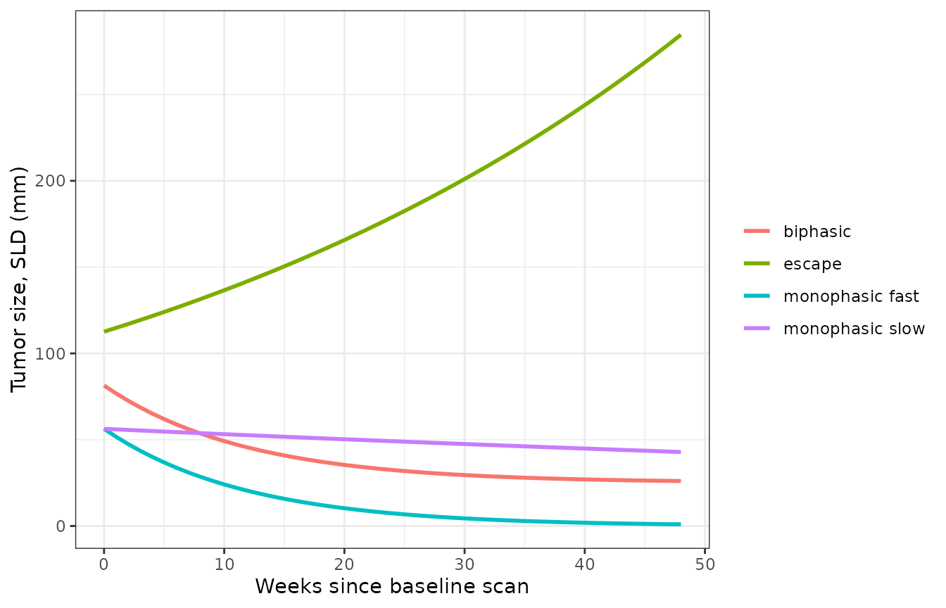

Typical-value tumor-size profiles for the four mixture classes. Replicates the patterns of Figure 1c and 1d of Chatterjee 2017.

The structural switches are exact identities, so they are asserted exactly.

arch0 <- mix_arch |> dplyr::filter(time == 0) |> dplyr::arrange(class)
mix_struct <- mix_arch |>
  dplyr::group_by(class) |>
  dplyr::summarise(TS0 = TS[time == 0], kdeath = kdeath[1], .groups = "drop")

stopifnot(
  # Escape: kill rate fixed to 0, no deep portion, shallow baseline x 2.00.
  isTRUE(all.equal(mix_struct$kdeath[mix_struct$class == "escape"], 0)),
  isTRUE(all.equal(mix_struct$TS0[mix_struct$class == "escape"], 2 * 56.3)),
  # Monophasic slow: base kill rate, no deep portion.
  isTRUE(all.equal(mix_struct$kdeath[mix_struct$class == "monophasic slow"], 3.57e-3)),
  isTRUE(all.equal(mix_struct$TS0[mix_struct$class == "monophasic slow"], 56.3)),
  # Biphasic: kill rate x 4.17 AND the only class carrying the deep portion.
  isTRUE(all.equal(mix_struct$kdeath[mix_struct$class == "biphasic"], 4.17 * 3.57e-3)),
  isTRUE(all.equal(mix_struct$TS0[mix_struct$class == "biphasic"], 56.3 + 25.1)),
  # Monophasic fast: same kill rate as biphasic, no deep portion.
  isTRUE(all.equal(mix_struct$kdeath[mix_struct$class == "monophasic fast"], 4.17 * 3.57e-3)),
  isTRUE(all.equal(mix_struct$TS0[mix_struct$class == "monophasic fast"], 56.3))
)

The solve must also reproduce the published closed form y(t) = BASEL1 * exp(KL * t - KD * t) + BASEL2 to machine precision, because both sides use the same drawn parameters and the model carries no ODE state.

mix_cf <- mix_arch |>
  dplyr::mutate(
    b1 = ifelse(class == "escape", 2 * 56.3, 56.3),
    b2 = ifelse(class == "biphasic", 25.1, 0),
    closed = b1 * exp((2.76e-3 - kdeath) * time) + b2
  )
stopifnot(max(abs(mix_cf$TS - mix_cf$closed)) < 1e-10)

The class probabilities

The second-stage multinomial regression is carried in the same file and returns the four class probabilities as derived outputs. At the source’s covariate centering values (AUCss-6weeks 6000 mg*day/L, no affected nodes, baseline SLD 98.15 mm) it must reproduce the P1-P4 row of supplementary Table 2B.

mp <- rxode2::rxSolve(mixz, rxode2::et(0), mix_ref, returnType = "data.frame")
#> ℹ omega/sigma items treated as zero: 'etalkdeath', 'etalrbase_shallow', 'etalrbase_deep', 'etalrv'
mix_prob <- c(mp$prob_escape, mp$prob_monophasic_slow, mp$prob_biphasic, mp$prob_monophasic_fast)
tibble::tibble(
  Class = c("escape", "monophasic slow", "biphasic", "monophasic fast"),
  Model = round(mix_prob, 4),
  `Supplementary Table 2B` = c(0.286, 0.396, 0.263, 0.0553)
) |>
  knitr::kable(caption = "Multinomial class probabilities at the source centering covariates.")

Multinomial class probabilities at the source centering covariates.
Class	Model	Supplementary Table 2B
escape	0.2859	0.2860
monophasic slow	0.3957	0.3960
biphasic	0.2630	0.2630
monophasic fast	0.0555	0.0553


stopifnot(
  isTRUE(all.equal(sum(mix_prob), 1)),
  # Published to three significant figures, so an absolute half-last-digit
  # tolerance rather than a percentage.
  max(abs(mix_prob - c(0.286, 0.396, 0.263, 0.0553))) < 5e-4
)

Main-article Table 2 reports a different set of class probabilities, from the covariate-free logits estimated inside the mixture run itself. Its footnote c says they are “derived from estimates of the logits and corrected for the frequency of patients with missing post-baseline scans” – patients with no post-baseline scan were assigned to the escape class a priori. That correction is an arithmetic identity, and recovering a single consistent missing-scan fraction from all three responder classes is a strong check on the transcription of both the logits and the probabilities.

t2_logit <- c(0.903, 0.48, -0.92)                 # Table 2, LGT2 / LGT3 / LGT4
t2_rep <- c(0.294, 0.389, 0.255, 0.0628)          # Table 2, P1 / P2 / P3 / P4
t2_raw <- c(1, exp(t2_logit)) / (1 + sum(exp(t2_logit)))

# Each responder class is shrunk by the same factor (1 - m); solve for m three
# independent ways.
m_implied <- 1 - t2_rep[-1] / t2_raw[-1]
m <- mean(m_implied)
p1_rebuilt <- m + (1 - m) * t2_raw[1]

tibble::tibble(
  Class = c("escape", "monophasic slow", "biphasic", "monophasic fast"),
  `Raw multinomial of Table 2 logits` = round(t2_raw, 4),
  `After missing-scan correction` = round(c(p1_rebuilt, (1 - m) * t2_raw[-1]), 4),
  `Table 2 as printed` = t2_rep
) |>
  knitr::kable(caption = "Table 2 class probabilities are the raw multinomial with the missing-post-baseline-scan fraction folded into the escape class.")

Table 2 class probabilities are the raw multinomial with the missing-post-baseline-scan fraction folded into the escape class.
Class	Raw multinomial of Table 2 logits	After missing-scan correction	Table 2 as printed
escape	0.1824	0.2933	0.2940
monophasic slow	0.4501	0.3890	0.3890
biphasic	0.2948	0.2548	0.2550
monophasic fast	0.0727	0.0628	0.0628


stopifnot(
  # All three responder classes imply the same missing-scan fraction.
  diff(range(m_implied)) < 0.005,
  # ...which lands at about 13.6% of the KEYNOTE-001 mixture dataset.
  m > 0.13, m < 0.14,
  # ...and rebuilds the reported escape probability.
  abs(p1_rebuilt - t2_rep[1]) < 0.002
)

Simulated response rates

The paper simulates response rates at week 28 from the mixture model combined with the multinomial regression (main-article Figure 3a). The cohort below follows the supplementary simulation methodology: draw a class per subject from the multinomial, then solve the tumor-size model with the full between-subject variability. Exposure is computed the way the source control stream computes it, AUCss-6weeks = dose * weight / CL * 6 / regimen, with the median clearance (0.2065 L/day) and median weight (78.9 kg) that the source multinomial control stream records for this cohort, and the between-subject clearance variance taken from the companion population-PK model packaged here as Ahamadi_2017_pembrolizumab.

Everything stochastic is drawn with base R’s generator under an explicit set.seed(), and the between-subject random effects are passed into rxSolve() as parameters, so the cohort is identical on every machine and every rxode2 build.

n_sub <- 200L
mvn_draw <- function(n, S) matrix(stats::rnorm(n * ncol(S)), n) %*% chol(S)

set.seed(20170129)
mix_e12 <- mvn_draw(n_sub, matrix(c(0.490796, 0.811621, 0.811621, 1.802122), 2))
mix_cl <- 0.2065 * exp(stats::rnorm(n_sub, 0, sqrt(0.134)))  # Ahamadi 2017 etalcl
mix_wt <- 78.9 * exp(stats::rnorm(n_sub, 0, 0.3144))
mix_u <- stats::runif(n_sub)

mix_cohort <- data.frame(
  id = seq_len(n_sub), NTARGET = 3, WHO_PS = 0, TUM_SLD = 98.15, NNODAL = 0,
  etalkdeath = stats::rnorm(n_sub, 0, sqrt(0.109392)),
  etalrbase_shallow = mix_e12[, 1], etalrbase_deep = mix_e12[, 2], etalrv = 0,
  MIX_MONO_SLOW = 0L, MIX_BIPHASIC = 0L, MIX_MONO_FAST = 0L
)
mix_cohort_ev <- rxode2::et(c(0, 28 * 7)) |> rxode2::et(id = seq_len(n_sub))

mix_orr <- function(dose_mgkg, regimen_wk) {
  p <- mix_cohort
  p$AUC_PEMBRO <- dose_mgkg * mix_wt / mix_cl * 6 / regimen_wk
  probs <- rxode2::rxSolve(mixz, mix_cohort_ev, p, returnType = "data.frame") |>
    dplyr::filter(time == 0) |>
    dplyr::select(prob_escape, prob_monophasic_slow, prob_biphasic, prob_monophasic_fast)
  k <- max.col(mix_u < t(apply(probs, 1, cumsum)), ties.method = "first")
  p$MIX_MONO_SLOW <- as.integer(k == 2L)
  p$MIX_BIPHASIC <- as.integer(k == 3L)
  p$MIX_MONO_FAST <- as.integer(k == 4L)
  s <- rxode2::rxSolve(mixz, mix_cohort_ev, p, returnType = "data.frame")
  cfb <- s$TS[s$time == 28 * 7] / s$TS[s$time == 0] - 1
  mean(cfb <= -0.30)
}

mix_arms <- tibble::tibble(dose = c(1, 2, 10, 10), regimen = c(3, 3, 3, 2)) |>
  dplyr::mutate(
    Regimen = paste0(dose, " mg/kg Q", regimen, "W"),
    raw = vapply(seq_along(dose), function(i) mix_orr(dose[i], regimen[i]), numeric(1)),
    corrected = raw * (1 - m)
  )
#> Warning: There were 8 warnings in `dplyr::mutate()`.
#> The first warning was:
#> ℹ In argument: `raw = vapply(...)`.
#> Caused by warning:
#> ! multi-subject simulation without without 'omega'
#> ℹ Run `dplyr::last_dplyr_warnings()` to see the 7 remaining warnings.

The paper’s simulated response rates come from the corrected class probabilities – the same missing-post-baseline-scan adjustment applied above – so the comparison must be made against the corrected column.

mix_arms |>
  dplyr::mutate(
    `Simulated ORR, raw` = sprintf("%.1f%%", 100 * raw),
    `Simulated ORR, missing-scan corrected` = sprintf("%.1f%%", 100 * corrected),
    `Published (90% CI)` = c("-", "32.9% (28.2-37.7)", "35.9% (31.1-40.4)", "-")
  ) |>
  dplyr::select(Regimen, `Simulated ORR, raw`,
                `Simulated ORR, missing-scan corrected`, `Published (90% CI)`) |>
  knitr::kable(caption = "Week-28 objective response rate, mixture model, versus Chatterjee 2017 Figure 3a.")

Week-28 objective response rate, mixture model, versus Chatterjee 2017 Figure 3a.
Regimen	Simulated ORR, raw	Simulated ORR, missing-scan corrected	Published (90% CI)
1 mg/kg Q3W	39.5%	34.1%	-
2 mg/kg Q3W	39.5%	34.1%	32.9% (28.2-37.7)
10 mg/kg Q3W	45.0%	38.9%	35.9% (31.1-40.4)
10 mg/kg Q2W	47.0%	40.6%	-


pub_mix <- c(`2 mg/kg Q3W` = 0.329, `10 mg/kg Q3W` = 0.359)
sim_mix <- setNames(mix_arms$corrected, mix_arms$Regimen)[names(pub_mix)]

stopifnot(
  # Centre: a mis-transcribed rate constant or baseline moves these by tens of
  # percent, so the tolerance is tight relative to that failure mode while
  # allowing for the covariate resampling the source used and this cohort does
  # not.
  max(abs(sim_mix - pub_mix)) < 0.07,
  # Flatness: the paper's whole conclusion is that the 5-fold dose range buys
  # almost nothing. Published difference 3.0 percentage points.
  sim_mix[["10 mg/kg Q3W"]] - sim_mix[["2 mg/kg Q3W"]] >= 0,
  sim_mix[["10 mg/kg Q3W"]] - sim_mix[["2 mg/kg Q3W"]] < 0.08
)

The consolidated model

Structure

conz <- rxode2::zeroRe(con)
con_ref <- data.frame(
  TUM_SLD = 80.75, AUC_PEMBRO = 7079, PRIOR_IPI = 0, PDL1_TUM_POS = 1,
  PDL1_TUM_MISSING = 0, TUM_BRAF_MUT = 0, T_SCAN_TO_DOSE = 0
)
con_ev <- rxode2::et(seq(0, 504, by = 7)) |> rxode2::et(amt = 0, cmt = "growth", time = 0)
con_strata <- list(
  "reference (IPI-naive, PD-L1+, BRAF wt)" = list(),
  "PD-L1 negative" = list(PDL1_TUM_POS = 0),
  "PD-L1 unknown" = list(PDL1_TUM_POS = 0, PDL1_TUM_MISSING = 1),
  "IPI-experienced" = list(PRIOR_IPI = 1),
  "BRAF mutant" = list(TUM_BRAF_MUT = 1),
  "baseline SLD 161.5 mm" = list(TUM_SLD = 161.5),
  "delay 42 days" = list(T_SCAN_TO_DOSE = 42)
)
con_arch <- lapply(names(con_strata), function(nm) {
  cv <- con_ref
  ch <- con_strata[[nm]]
  if (length(ch)) cv[names(ch)] <- ch
  # Tight solver tolerances so the closed-form gate below measures the
  # encoding, not the integrator.
  s <- rxode2::rxSolve(conz, con_ev, cv, atol = 1e-12, rtol = 1e-12,
                       returnType = "data.frame")
  data.frame(stratum = nm, time = s$time, TS = s$TS, baseline = cv$TUM_SLD,
             kgrowth = s$kgrowth[1], kdeath = s$kdeath[1], fresp = s$fresp[1])
}) |> dplyr::bind_rows()
#> ℹ omega/sigma items treated as zero: 'etalkgrowth', 'etalkdeath', 'etalogitfresp'
#> ℹ omega/sigma items treated as zero: 'etalkgrowth', 'etalkdeath', 'etalogitfresp'
#> ℹ omega/sigma items treated as zero: 'etalkgrowth', 'etalkdeath', 'etalogitfresp'
#> ℹ omega/sigma items treated as zero: 'etalkgrowth', 'etalkdeath', 'etalogitfresp'
#> ℹ omega/sigma items treated as zero: 'etalkgrowth', 'etalkdeath', 'etalogitfresp'
#> ℹ omega/sigma items treated as zero: 'etalkgrowth', 'etalkdeath', 'etalogitfresp'
#> ℹ omega/sigma items treated as zero: 'etalkgrowth', 'etalkdeath', 'etalogitfresp'

ggplot2::ggplot(con_arch, ggplot2::aes(time / 7, 100 * (TS / baseline - 1), colour = stratum)) +
  ggplot2::geom_line(linewidth = 0.9) +
  ggplot2::geom_hline(yintercept = c(-30, 20), linetype = "dashed", colour = "grey40") +
  ggplot2::labs(x = "Weeks since baseline scan", y = "Change from baseline in SLD (%)", colour = NULL) +
  ggplot2::theme_bw()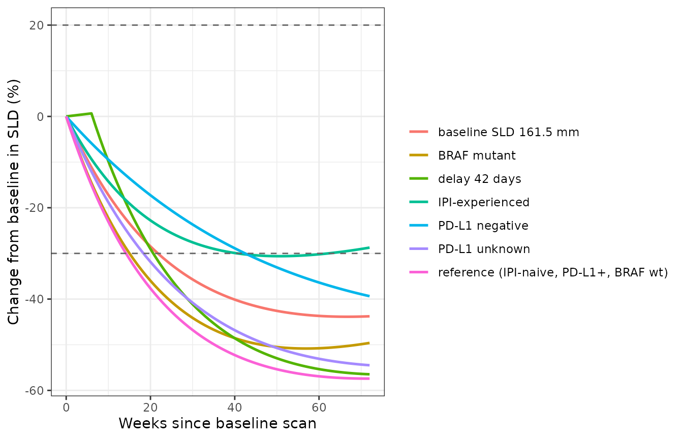

Typical-value consolidated-model profiles across the retained covariate strata, at the median baseline SLD of 80.75 mm and the reference exposure of 7079 mg*day/L. Replicates the range of patterns in Figure 1b of Chatterjee 2017.

Two exact structural identities, then every retained covariate effect checked against the value supplementary Table 4C prints.

con_p <- con_arch |>
  dplyr::group_by(stratum) |>
  dplyr::summarise(TS0 = TS[time == 0], baseline = baseline[1],
                   kgrowth = kgrowth[1], kdeath = kdeath[1], fresp = fresp[1],
                   .groups = "drop")
g <- function(nm, col) con_p[[col]][con_p$stratum == nm]
ref <- "reference (IPI-naive, PD-L1+, BRAF wt)"

stopifnot(
  # TS(0) must equal the observed baseline covariate exactly, for every
  # stratum -- that is what makes TUM_SLD a regressor rather than a parameter.
  isTRUE(all.equal(con_p$TS0, con_p$baseline)),
  # Reference typical values equal supplementary Table 4C as printed.
  isTRUE(all.equal(g(ref, "kgrowth"), 0.000512)),
  isTRUE(all.equal(g(ref, "kdeath"), 0.00609)),
  isTRUE(all.equal(g(ref, "fresp"), 0.696)),
  # Categorical fractional deviations.
  isTRUE(all.equal(g("BRAF mutant", "kgrowth"), 0.000512 * (1 + 0.702))),
  isTRUE(all.equal(g("PD-L1 negative", "kdeath"), 0.00609 * (1 - 0.614))),
  isTRUE(all.equal(g("PD-L1 unknown", "kdeath"), 0.00609 * (1 - 0.21))),
  # Additive deviation on the logit of f.
  isTRUE(all.equal(g("IPI-experienced", "fresp"), plogis(qlogis(0.696) - 0.964))),
  # Continuous effects of baseline tumor size: power on kdeath, linear on
  # logit(f), both centered at 80.75 mm.
  isTRUE(all.equal(g("baseline SLD 161.5 mm", "kdeath"), 0.00609 * 2^-0.186)),
  isTRUE(all.equal(g("baseline SLD 161.5 mm", "fresp"),
                   plogis(qlogis(0.696) - 0.00541 * (161.5 - 80.75))))
)

The delay term must hold the accessible sub-state flat until T_SCAN_TO_DOSE, after which the profile is the un-delayed one shifted in time.

d0 <- con_arch |> dplyr::filter(stratum == ref) |> dplyr::arrange(time)
d42 <- con_arch |> dplyr::filter(stratum == "delay 42 days") |> dplyr::arrange(time)
shrink0 <- 80.75 * 0.696 * exp(-0.00609 * pmax(0, d0$time))
shrink42 <- 80.75 * 0.696 * exp(-0.00609 * pmax(0, d42$time - 42))
grow <- 80.75 * (1 - 0.696) * exp(0.000512 * d0$time)

stopifnot(
  # Both sides use the same parameters, so the only difference is ODE
  # integration error; asserted as a relative tolerance at the solver
  # tolerances requested above.
  max(abs(d0$TS - (shrink0 + grow)) / d0$TS) < 1e-9,
  max(abs(d42$TS - (shrink42 + grow)) / d42$TS) < 1e-9,
  # Before the delay the only motion is the resistant fraction growing.
  all(diff(d42$TS[d42$time <= 42]) > 0)
)

Exposure-response flatness

Both exposure exponents are small and neither is statistically significant (P = 0.20 for ipilimumab-naive, P = 0.25 for ipilimumab-experienced). Because AUCss-6weeks is proportional to the mg/kg dose, the kill-rate ratio across the studied fivefold dose range is a closed-form number.

ratio <- function(ipi) {
  cv <- con_ref
  cv$PRIOR_IPI <- ipi
  k <- vapply(c(1, 5), function(f) {
    cv$AUC_PEMBRO <- 7079 * f
    rxode2::rxSolve(conz, rxode2::et(0), cv, returnType = "data.frame")$kdeath[1]
  }, numeric(1))
  k[2] / k[1]
}
tibble::tibble(
  Stratum = c("ipilimumab-naive", "ipilimumab-experienced"),
  `kdeath ratio, 10 vs 2 mg/kg` = round(c(ratio(0), ratio(1)), 4),
  `Closed form` = round(c(5^0.131, 5^0.1), 4)
) |>
  knitr::kable(caption = "A fivefold increase in exposure raises the tumor kill rate by less than a quarter.")
#> ℹ omega/sigma items treated as zero: 'etalkgrowth', 'etalkdeath', 'etalogitfresp'
#> ℹ omega/sigma items treated as zero: 'etalkgrowth', 'etalkdeath', 'etalogitfresp'
#> ℹ omega/sigma items treated as zero: 'etalkgrowth', 'etalkdeath', 'etalogitfresp'
#> ℹ omega/sigma items treated as zero: 'etalkgrowth', 'etalkdeath', 'etalogitfresp'

A fivefold increase in exposure raises the tumor kill rate by less than a quarter.
Stratum	kdeath ratio, 10 vs 2 mg/kg	Closed form
ipilimumab-naive	1.2347	1.2347
ipilimumab-experienced	1.1746	1.1746


stopifnot(
  isTRUE(all.equal(ratio(0), 5^0.131)),
  isTRUE(all.equal(ratio(1), 5^0.1)),
  # The paper's qualitative claim, asserted rather than left as prose: a
  # fivefold dose increase buys under 25% more kill rate in either stratum.
  ratio(0) < 1.25, ratio(1) < 1.25
)
#> ℹ omega/sigma items treated as zero: 'etalkgrowth', 'etalkdeath', 'etalogitfresp'
#> ℹ omega/sigma items treated as zero: 'etalkgrowth', 'etalkdeath', 'etalogitfresp'
#> ℹ omega/sigma items treated as zero: 'etalkgrowth', 'etalkdeath', 'etalogitfresp'
#> ℹ omega/sigma items treated as zero: 'etalkgrowth', 'etalkdeath', 'etalogitfresp'
#> ℹ omega/sigma items treated as zero: 'etalkgrowth', 'etalkdeath', 'etalogitfresp'
#> ℹ omega/sigma items treated as zero: 'etalkgrowth', 'etalkdeath', 'etalogitfresp'
#> ℹ omega/sigma items treated as zero: 'etalkgrowth', 'etalkdeath', 'etalogitfresp'
#> ℹ omega/sigma items treated as zero: 'etalkgrowth', 'etalkdeath', 'etalogitfresp'

Virtual cohort and simulated response rates

set.seed(20170129)
con_e3 <- mvn_draw(n_sub, matrix(c(1.64, -1.24, -1.54,
                                   -1.24, 1.39, 1.07,
                                   -1.54, 1.07, 5.53), 3, byrow = TRUE))
con_sld <- 80.60 * exp(stats::rnorm(n_sub, 0, 0.78))
con_wt <- 79.30 * exp(stats::rnorm(n_sub, 0, 0.3144))
con_cl_eta <- stats::rnorm(n_sub, 0, sqrt(0.134))
con_pdl1 <- sample(c("pos", "neg", "unk"), n_sub, TRUE, c(0.5410, 0.1647, 0.2943))
con_braf <- stats::rbinom(n_sub, 1, 0.2709)

# Calibrate the typical clearance so that the median 10 mg/kg Q3W exposure is
# the 7079 mg*day/L the source control stream names as exactly that quantity.
con_cl_typ <- 2 * 10 * 79.30 / 7079

con_cohort <- data.frame(
  id = seq_len(n_sub), TUM_SLD = con_sld, T_SCAN_TO_DOSE = 0,
  PDL1_TUM_POS = as.integer(con_pdl1 == "pos"),
  PDL1_TUM_MISSING = as.integer(con_pdl1 == "unk"),
  TUM_BRAF_MUT = con_braf,
  etalkgrowth = con_e3[, 1], etalkdeath = con_e3[, 2], etalogitfresp = con_e3[, 3]
)
con_cohort_ev <- rxode2::et(seq(0, 24 * 7, by = 7)) |>
  rxode2::et(amt = 0, cmt = "growth", time = 0) |>
  rxode2::et(id = seq_len(n_sub))

con_solve <- function(dose_mgkg, regimen_wk, ipi) {
  p <- con_cohort
  p$PRIOR_IPI <- ipi
  p$AUC_PEMBRO <- dose_mgkg * con_wt / (con_cl_typ * exp(con_cl_eta)) * 6 / regimen_wk
  rxode2::rxSolve(conz, con_cohort_ev, p, returnType = "data.frame")
}
con_orr <- function(dose_mgkg, regimen_wk, ipi) {
  s <- con_solve(dose_mgkg, regimen_wk, ipi)
  cfb <- s$TS[s$time == 24 * 7] / s$TS[s$time == 0] - 1
  mean(cfb <= -0.30)
}

con_arms <- tidyr::expand_grid(
  ipi = c(0L, 1L),
  tibble::tibble(dose = c(1, 2, 10, 10), regimen = c(3, 3, 3, 2))
) |>
  dplyr::mutate(
    Stratum = ifelse(ipi == 0L, "ipilimumab-naive", "ipilimumab-experienced"),
    Regimen = paste0(dose, " mg/kg Q", regimen, "W"),
    orr = vapply(seq_along(dose), function(i) con_orr(dose[i], regimen[i], ipi[i]), numeric(1))
  )
#> Warning: There were 8 warnings in `dplyr::mutate()`.
#> The first warning was:
#> ℹ In argument: `orr = vapply(...)`.
#> Caused by warning:
#> ! multi-subject simulation without without 'omega'
#> ℹ Run `dplyr::last_dplyr_warnings()` to see the 7 remaining warnings.

con_pub <- tibble::tribble(
  ~Stratum, ~Regimen, ~Published,
  "ipilimumab-naive", "2 mg/kg Q3W", "44.7% (38.8-49.8)",
  "ipilimumab-naive", "10 mg/kg Q3W", "47.4% (43.7-51.3)",
  "ipilimumab-experienced", "2 mg/kg Q3W", "36.9% (32.8-41.3)",
  "ipilimumab-experienced", "10 mg/kg Q3W", "38.8% (35.2-42.7)"
)
con_arms |>
  dplyr::mutate(`Simulated ORR` = sprintf("%.1f%%", 100 * orr)) |>
  dplyr::left_join(con_pub, by = c("Stratum", "Regimen")) |>
  dplyr::mutate(`Published (90% CI)` = tidyr::replace_na(Published, "-")) |>
  dplyr::select(Stratum, Regimen, `Simulated ORR`, `Published (90% CI)`) |>
  knitr::kable(caption = "Week-24 objective response rate, consolidated model, versus Chatterjee 2017 Figure 3b and 3c.")

Week-24 objective response rate, consolidated model, versus Chatterjee 2017 Figure 3b and 3c.
Stratum	Regimen	Simulated ORR	Published (90% CI)
ipilimumab-naive	1 mg/kg Q3W	44.5%	-
ipilimumab-naive	2 mg/kg Q3W	45.0%	44.7% (38.8-49.8)
ipilimumab-naive	10 mg/kg Q3W	46.0%	47.4% (43.7-51.3)
ipilimumab-naive	10 mg/kg Q2W	47.0%	-
ipilimumab-experienced	1 mg/kg Q3W	33.5%	-
ipilimumab-experienced	2 mg/kg Q3W	34.5%	36.9% (32.8-41.3)
ipilimumab-experienced	10 mg/kg Q3W	37.5%	38.8% (35.2-42.7)
ipilimumab-experienced	10 mg/kg Q2W	38.0%	-

pick <- function(st, rg) con_arms$orr[con_arms$Stratum == st & con_arms$Regimen == rg]
sim_con <- c(
  naive_2 = pick("ipilimumab-naive", "2 mg/kg Q3W"),
  naive_10 = pick("ipilimumab-naive", "10 mg/kg Q3W"),
  exp_2 = pick("ipilimumab-experienced", "2 mg/kg Q3W"),
  exp_10 = pick("ipilimumab-experienced", "10 mg/kg Q3W")
)
pub_con <- c(naive_2 = 0.447, naive_10 = 0.474, exp_2 = 0.369, exp_10 = 0.388)

stopifnot(
  # Centre: every arm within 7 percentage points of the paper's own simulation.
  max(abs(sim_con - pub_con)) < 0.07,
  # Direction: ipilimumab-naive patients respond better in both dose groups.
  # Evaluated on the SAME simulated subjects with only PRIOR_IPI flipped, so
  # this is a paired comparison and carries no sampling noise.
  sim_con[["naive_2"]] > sim_con[["exp_2"]],
  sim_con[["naive_10"]] > sim_con[["exp_10"]],
  # Flatness again: published gaps are 2.7 and 1.9 percentage points.
  sim_con[["naive_10"]] - sim_con[["naive_2"]] >= 0,
  sim_con[["exp_10"]] - sim_con[["exp_2"]] >= 0,
  max(sim_con[["naive_10"]] - sim_con[["naive_2"]],
      sim_con[["exp_10"]] - sim_con[["exp_2"]]) < 0.08
)

con_traj <- dplyr::bind_rows(
  con_solve(10, 3, 0L) |> dplyr::mutate(Stratum = "ipilimumab-naive"),
  con_solve(10, 3, 1L) |> dplyr::mutate(Stratum = "ipilimumab-experienced")
) |>
  dplyr::group_by(Stratum, time) |>
  dplyr::summarise(
    p10 = quantile(TS, 0.10), p50 = median(TS), p90 = quantile(TS, 0.90),
    .groups = "drop"
  )
#> Warning: multi-subject simulation without without 'omega'
#> Warning: multi-subject simulation without without 'omega'

ggplot2::ggplot(con_traj, ggplot2::aes(time / 7, p50, colour = Stratum, fill = Stratum)) +
  ggplot2::geom_ribbon(ggplot2::aes(ymin = p10, ymax = p90), alpha = 0.15, colour = NA) +
  ggplot2::geom_line(linewidth = 1) +
  ggplot2::labs(x = "Weeks since baseline scan", y = "Tumor size, SLD (mm)",
                colour = NULL, fill = NULL) +
  ggplot2::theme_bw()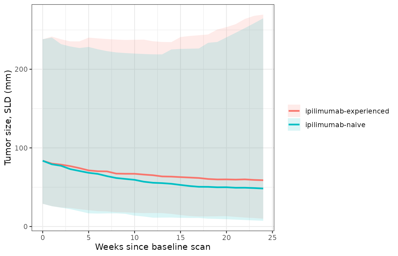

Simulated tumor-size trajectories at 10 mg/kg Q3W, median with the 10th and 90th percentiles, by prior-ipilimumab status. The corresponding observed-versus-predicted display is Figure 2e and 2f of Chatterjee 2017.

Comparison against the published simulations

tibble::tibble(
  Model = c(rep("mixture (week 28)", 2), rep("consolidated (week 24)", 4)),
  Arm = c("2 mg/kg Q3W", "10 mg/kg Q3W",
          "IPI-naive, 2 mg/kg Q3W", "IPI-naive, 10 mg/kg Q3W",
          "IPI-experienced, 2 mg/kg Q3W", "IPI-experienced, 10 mg/kg Q3W"),
  Simulated = sprintf("%.1f%%", 100 * c(sim_mix, sim_con)),
  Published = sprintf("%.1f%%", 100 * c(pub_mix, pub_con)),
  `Difference (percentage points)` = sprintf("%+.1f", 100 * (c(sim_mix, sim_con) - c(pub_mix, pub_con)))
) |>
  knitr::kable(caption = "Objective response rate: this reconstruction versus the source paper's own trial simulations.")

Objective response rate: this reconstruction versus the source paper’s own trial simulations.
Model	Arm	Simulated	Published	Difference (percentage points)
mixture (week 28)	2 mg/kg Q3W	34.1%	32.9%	+1.2
mixture (week 28)	10 mg/kg Q3W	38.9%	35.9%	+3.0
consolidated (week 24)	IPI-naive, 2 mg/kg Q3W	45.0%	44.7%	+0.3
consolidated (week 24)	IPI-naive, 10 mg/kg Q3W	46.0%	47.4%	-1.4
consolidated (week 24)	IPI-experienced, 2 mg/kg Q3W	34.5%	36.9%	-2.4
consolidated (week 24)	IPI-experienced, 10 mg/kg Q3W	37.5%	38.8%	-1.3

Assumptions and deviations

No PKNCA validation. Neither model produces a concentration or takes a dosing event, so there is nothing for non-compartmental analysis to integrate. Validation is structural plus a reproduction of the paper’s own simulated response rates.
Exposure distribution. The source resampled AUCss-6weeks with replacement from the observed dataset, which preserves the correlation between exposure and the other covariates. That dataset is not available, so both cohorts here compute exposure from the source’s own formula dose * weight / CL * 6 / regimen with independently drawn weight and clearance. For the mixture cohort the median clearance (0.2065 L/day) and median weight (78.9 kg) are the values the source multinomial control stream records. For the consolidated cohort the typical clearance is calibrated so the median 10 mg/kg Q3W exposure is 7079 mg*day/L, which is what the source control stream comment says that constant is. In both cases the between-subject clearance variance (omega^2 = 0.134, 37.9% CV) is taken from the companion population-PK model Ahamadi_2017_pembrolizumab, not invented.
Covariate distributions. Baseline SLD and weight are drawn log-normally with the medians from supplementary Table 5B and a log-scale SD chosen so the 0.1st and 99.9th percentiles approximately span the reported ranges; the paper reports only median and range, not a distributional form. PD-L1 status and BRAF status are drawn from the marginal frequencies in supplementary Table 5A, independently of each other and of tumor size – the source resampling would have preserved any association between them.
Mixture-model covariates are held at the source centering values. The paper reports covariate distributions only for the consolidated dataset (supplementary Table 5), so the mixture cohort uses NTARGET = 3, ECOG = 0, baseline SLD = 98.15 mm and no affected nodes – the centering constants in the source control stream. The multinomial class probabilities are then exactly the supplementary Table 2B typical values, which is why the raw simulated response rate has to be corrected by the same missing-post-baseline-scan factor the paper folds into its Table 2 probabilities before it can be compared with the published figure.
T_SCAN_TO_DOSE = 0. The source carries a per-subject delay column but never reports its distribution, so the cohorts assume shrinkage begins at the baseline scan. The delay gate above exercises a non-zero value.
No between-subject variability on the mixture model’s growth rate. The source control stream declares $OMEGA 0 FIX ; IIV_KL and Table 2 reports no IIV row for KL, so no eta is written for lkgrowth. A zero-variance eta is omitted rather than encoded as fixed(0) because a singular OMEGA block breaks rxode2’s Cholesky decomposition at solve time.
ETA_EPS heading. Main-article Table 2 labels the between-subject variability of the residual error “(variance)” while supplementary Table 2A labels the same row “%CV”. The control stream’s $OMEGA 0.0625 initial back-transforms to 25.4% CV under the tables’ own footnote formula CV% = 100 * sqrt(exp(omega^2) - 1), which matches the reported 26.1 / 26.4 as a CV, not as a variance. The model file reads it as a CV and says so.
Residual error is applied on the log scale. The source fits log(SLD) with W = sqrt(propSd^2 + addSd^2 / SLD^2) and $SIGMA 1 FIX, so the packaged model uses TS ~ lnorm(sdlog) with sdlog computed in model(). The source’s floors on W (0.01) and on the prediction (1e-5) cannot bind at the published parameter values and are not reproduced.
The VPC censoring rule is not in the model. Figure 2e and 2f censor simulated patients whose tumors exceeded threefold baseline after at least six months on treatment, to mimic study withdrawal. That is post-processing for the visual predictive check, not model structure, so it is not encoded. The paper itself notes the rule is probably too lenient and contributes to the modest over-prediction of the 90th percentile.
Base models not packaged. Supplementary Tables 2A and 4A report base (covariate-free) versions of both models. Per library policy only the final models are packaged.
Second-stage multinomial folded into the mixture file. The source fit the class-probability covariate model as a separate NONMEM run, because patients without a post-baseline scan were assigned to the escape class a priori and could not contribute to a joint estimation. It is carried in the same model file here because its only purpose is to assign a class before the tumor-size model can be solved, and its parameters are the covariate-containing stage of one model’s covariate search rather than an independent model. The covariate-free logits that main-article Table 2 reports from the mixture run itself are therefore not in ini(); they are exercised in the Table 2 correction gate above.
Statistical significance. Neither exposure exponent in the consolidated model, and no exposure term at all in the final mixture model, is a significant predictor of tumor shrinkage. The authors retained the consolidated exponents only so the magnitude of a potential relationship could be simulated. Treat them as an uncertainty-visualisation device, not as an established exposure-response relationship.